.ipynb .pdf

Binder

Contents

import matplotlib.pyplot as plt
import numpy as np
from statsmodels.tsa.arima_process import arma_acovf
from scipy.linalg import toeplitz

from matplotlib import rc
rc('font',**{'family':'serif','serif':['Palatino']})
rc('text', usetex=True)


plt.rcParams.update({'ytick.left' : True,
                     "xtick.bottom" : True,
                     "ytick.major.size": 0,
                     "ytick.major.width": 0,
                     "xtick.major.size": 0,
                     "xtick.major.width": 0,
                     "ytick.direction": 'in',
                     "xtick.direction": 'in',
                     'ytick.major.right': False,
                     'xtick.major.top': True,
                     'xtick.top': True,
                     'ytick.right': True,
                     'ytick.labelsize': 18,
                     'xtick.labelsize': 18
                    })

def correlation_from_covariance(covariance):
    v = np.sqrt(np.diag(covariance))
    outer_v = np.outer(v, v)
    correlation = covariance / outer_v
    correlation[covariance == 0] = 0
    return correlation

n_obs = 20
arparams = np.array([.80])
maparams = np.array([0])
ar = np.r_[1, -arparams] # add zero-lag and negate
ma = np.r_[1, maparams] # add zero-lag
sigma2=np.array([1])

acov = arma_acovf(ar=ar, ma=ma, nobs=n_obs, sigma2=sigma2)

Sigma = toeplitz(acov)

corr = correlation_from_covariance(Sigma)

tmp = np.random.rand(n_obs, n_obs)
unrestr_cov = np.dot(tmp,tmp.T)

unrestr_mean = np.random.rand(n_obs, 1)

def show_covariance(mean_vec, cov_mat):
    K = cov_mat.shape[0]
    
    fig, ax = plt.subplots(nrows=1, ncols=2, figsize=(20,8))

    m = ax[0].imshow(mean_vec,
                       cmap='GnBu',
                      )

    K = Sigma.shape[0]

    ax[0].set_xticks([])
    ax[0].set_xticklabels([]);
    ax[0].set_yticks(range(0,K))
    ax[0].set_yticklabels(range(1, K+1));

    #ax[0].set_xlabel('$\mu$', fontsize=24)
    ax[0].set_title('mean', fontsize=24)

    c = ax[1].imshow(cov_mat,
                       cmap="inferno",
                      )
    plt.colorbar(c);


    ax[1].set_xticks(range(0,K))
    ax[1].set_xticklabels(range(1, K+1));
    ax[1].set_yticks(range(0,K))
    ax[1].set_yticklabels(range(1, K+1));  
    ax[1].set_title('Covariance', fontsize=24)

    plt.subplots_adjust(wspace=-0.7)

    #return (fig, ax)

Time series vs. cross-section

• sample of households at a point in time (income, expenditure)

• aggregate (income, expenditure) over time

• dependent vs. independent sampling

$$\begin{array}{r}\left[\begin{array}{c}{Z}_1\\ Z_2\\ Z_3\\ ⋮\\ Z_K\end{array}\right]\end{array}$$

• $Z_i$ can be a scalar, or a vector, e.g.

$$\begin{array}{r}{Z}_i=\left[\begin{array}{c}{y}_i\\ X_i\end{array}\right]\end{array}$$

$$Z\sim \mathcal{N}(\mu ,\mathrm{\Sigma })$$

$$\begin{array}{r}\left[\begin{array}{c}{Z}_1\\ Z_2\\ Z_3\\ ⋮\\ Z_K\end{array}\right]\sim \mathcal{N}(\left[\begin{array}{c}{\mu }_1\\ {\mu }_2\\ {\mu }_3\\ ⋮\\ {\mu }_K\end{array}\right],\left(\begin{array}{ccccc}\mathrm{\Sigma }(1,1)& \mathrm{\Sigma }(1,2)& \mathrm{\Sigma }(1,3)& \cdots & \mathrm{\Sigma }(1,K)\\ \mathrm{\Sigma }(2,1)& \mathrm{\Sigma }(2,2)& \mathrm{\Sigma }(2,3)& \cdots & ⋮\\ \mathrm{\Sigma }(3,1)& \mathrm{\Sigma }(3,2)& \mathrm{\Sigma }(3,3)& \cdots & ⋮\\ ⋮& ⋮& ⋮& \cdots & ⋮\\ \mathrm{\Sigma }(K,1)& \cdots & \cdots & \cdots & \mathrm{\Sigma }(K,K)\end{array}\right))\end{array}$$

show_covariance(mean_vec=unrestr_mean, cov_mat=unrestr_cov)

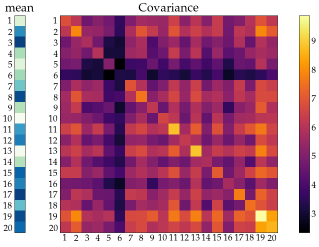
remember: symmetry of $\mathrm{\Sigma }$

Hopeless without resrtictions - structure on $\mu ,\mathrm{\Sigma }$

• independent

$$\begin{array}{r}\left[\begin{array}{c}{Z}_1\\ Z_2\\ Z_3\\ ⋮\\ Z_K\end{array}\right]\sim \mathcal{N}(\left[\begin{array}{c}{\mu }_1\\ {\mu }_2\\ {\mu }_3\\ ⋮\\ {\mu }_K\end{array}\right],\left(\begin{array}{ccccc}\mathrm{\Sigma }(1,1)& 0& 0& \cdots & 0\\ 0& \mathrm{\Sigma }(2,2)& 0& \cdots & ⋮\\ 0& 0& \mathrm{\Sigma }(3,3)& \cdots & ⋮\\ ⋮& ⋮& ⋮& \cdots & ⋮\\ 0& \cdots & \cdots & \cdots & \mathrm{\Sigma }(K,K)\end{array}\right))\end{array}$$

show_covariance(mean_vec=unrestr_mean, cov_mat=np.diagflat(unrestr_cov.diagonal()))

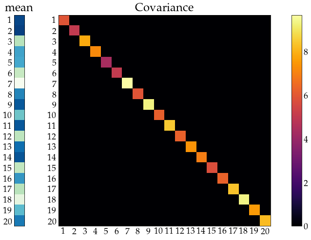
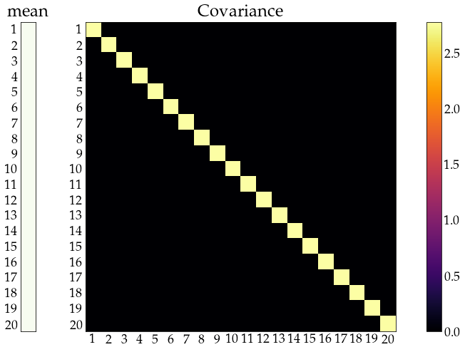
• … and identically distributed

$$\begin{array}{r}\left[\begin{array}{c}{Z}_1\\ Z_2\\ Z_3\\ ⋮\\ Z_K\end{array}\right]\sim \mathcal{N}(\left[\begin{array}{c}\mu \\ \mu \\ \mu \\ ⋮\\ \mu \end{array}\right],\left(\begin{array}{ccccc}\mathrm{\Sigma }& 0& 0& \cdots & 0\\ 0& \mathrm{\Sigma }& 0& \cdots & ⋮\\ 0& 0& \mathrm{\Sigma }& \cdots & ⋮\\ ⋮& ⋮& ⋮& \cdots & ⋮\\ 0& \cdots & \cdots & \cdots & \mathrm{\Sigma }\end{array}\right))\end{array}$$

Note: small $\mu$ and $\mathrm{\Sigma }$ - not the moments of full joint distribution above

show_covariance(mean_vec=np.ones((n_obs, 1)) ,cov_mat=np.diagflat(Sigma.diagonal()));

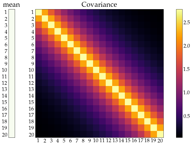
time series

• distribution ($\mu$, and $\mathrm{\Sigma }$) is time-invariant (stationarity)

• dependence - not too strong and weaker for distant elements (ergodicity)

show_covariance(mean_vec=np.ones((n_obs, 1)) ,cov_mat=Sigma);

time series models

• represent temporal dependence in a parsimonious way

  • AR (1) model:

  $$z_t=\alpha z_{t-1}+{\epsilon }_t$$

  • MA(1) model:

  $$z_t={\epsilon }_t+\psi {\epsilon }_{t-1}$$

  • ARMA(1,1) model:

  $$z_t=\alpha z_{t-1}+{\epsilon }_t+\psi {\epsilon }_{t-1}$$

  • etc.

• represent temporal interdependence among multiple variables in a parsimonious way

  • VAR (1) model

  • VMA(1) model

  • VARMA(1,1) model

  • etc.

Consequence of dependence

• information accumulates more slowly - need different statistical theory to justify methods

• forecast the future using the past

previous

Introduction

next

Time series concepts and models