.ipynb .pdf

Binder

Contents

ARCH

import warnings
warnings.simplefilter("ignore", FutureWarning)

import matplotlib.pyplot as plt
import seaborn as sns
sns.set_theme()
sns.set_context("notebook")

import pandas as pd
import sqlite3

Conditional heteroskedasticity

Time series models are (largely) models of the temporal dependence observed in time series data

• the future depends of the past

• the past is informative about the future

$$p(z_{t+h}|z_t,z_{t-1},\cdots )\ne p(z_{t+h})$$

Central objective of time series modeling is characterizing temporal dependence, i.e. characterizing

$$p(z_{t+h}|z_t,z_{t-1},\cdots )$$

or characterizing some of its moments, such as

$$\begin{array}{r}\begin{array}{c}\mathrm{E}(z_{t+h}|z_t,z_{t-1},\cdots )={\mathrm{E}}_t(z_{t+h})\\ \mathrm{var}(z_{t+h}|z_t,z_{t-1},\cdots )={\mathrm{var}}_t(z_{t+h})\end{array}\end{array}$$

So far, we have seen models for the conditional mean.

• for example, in $z_t=\alpha z_{t-1}+{\epsilon }_t$ the conditional mean is

$$\mathrm{E}(z_{t+1}|z_t,z_{t-1},\cdots )=\mathrm{E}(z_{t+1}|z_t)=\alpha z_t$$

changes with $z_t$

However, the assumptions about ${\epsilon }_t$ imply that $\mathrm{var}(z_{t+h}|z_t,z_{t-1},\cdots )$ is a constant (independent of $z_t,z_{t-1},\cdots$)

• for example, in $z_t=\alpha z_{t-1}+{\epsilon }_t$

$$\mathrm{var}(z_{t+1}|z_t,z_{t-1},\cdots )=\mathrm{var}({\epsilon }_{t+1}|z_t)=\mathrm{var}({\epsilon }_{t+1})={\sigma }^2$$

independent of $z_t$

Gaussian time series model

$$p(\underset{{\mathbf{z}}_1}{\underbrace{z_1,z_2,\cdots ,z_T}},\underset{{\mathbf{z}}_2}{\underbrace{z_{T+1},\cdots ,z_{T+h}}})=p({\mathbf{z}}_1,{\mathbf{z}}_2)\sim \mathcal{N}(\mathit{\mu },\mathbf{\Sigma }).$$

Forecasts

$$p({\mathbf{z}}_2|{\mathbf{z}}_1)=\mathcal{N}({\mathit{\mu }}_2+{\mathbf{\Sigma }}_{21}{\mathbf{\Sigma }}_{11}^{-1}({\mathbf{z}}_1-{\mathit{\mu }}_1),{\mathbf{\Sigma }}_{22}-{\mathbf{\Sigma }}_{21}{\mathbf{\Sigma }}_{11}^{-1}{\mathbf{\Sigma }}_{12})$$

• $\mathrm{E}({\mathbf{z}}_2|{\mathbf{z}}_1)={\mathit{\mu }}_2+{\mathbf{\Sigma }}_{21}{\mathbf{\Sigma }}_{11}^{-1}({\mathbf{z}}_1-{\mathit{\mu }}_1)$ function of ${\mathbf{z}}_1$

• $\mathrm{cov}({\mathbf{z}}_2|{\mathbf{z}}_1)={\mathbf{\Sigma }}_{22}-{\mathbf{\Sigma }}_{21}{\mathbf{\Sigma }}_{11}^{-1}{\mathbf{\Sigma }}_{12}$ constant

More generally, if

$$\begin{array}{r}{\epsilon }_t=z_t-\mathrm{E}(z_t|z_{t-1},z_{t-2},\cdots )\end{array}$$

then

$$\mathrm{E}({\epsilon }_t|z_{t-1},z_{t-2},\cdots )=0$$

and

$$\mathrm{E}({\epsilon }_t^2|z_{t-1},z_{t-2},\cdots )=\mathrm{var}({\epsilon }_t|z_{t-1},z_{t-2},\cdots )=\mathrm{var}(z_t|z_{t-1},z_{t-2},\cdots )$$

For $\mathrm{var}(z_t|z_{t-1},z_{t-2},\cdots )$ to vary with $(z_{t-1},z_{t-2},\cdots )$, we need $\mathrm{var}({\epsilon }_t|z_{t-1},z_{t-2},\cdots )$ to be a function of $(z_{t-1},z_{t-2},\cdots )$

$$\begin{array}{r}\begin{array}{rl}\mathrm{var}({\epsilon }_t|z_{t-1},z_{t-2},\cdots )& =\mathrm{E}({\epsilon }_t^2|z_{t-1},z_{t-2},\cdots )=h(z_{t-1},z_{t-2},\cdots )={\sigma }_t^2\end{array}\end{array}$$

where $h(.)$ is non-negative

and therefore

$$\mathrm{var}(z_t|z_{t-1},z_{t-2},\cdots )={\sigma }_t^2$$

conditional heteroskedasticity models are models for ${\sigma }_t^2$

• ${\sigma }_t^2={\sigma }^2$ - homoskedasticity

• ${\sigma }_t^2\ne {\sigma }^2$ - heteroskedasticity

Autoregressive conditional heteroskedasticity (ARCH) models

ARCH(1)

$${\sigma }_t^2={\omega }_0+{\omega }_1{\epsilon }_{t-1}^2$$

• ${\omega }_0>0$, ${\omega }_1\ge 0$ (for ${\sigma }_t^2$ to be positive)

• large shocks (${\epsilon }_{t-1}$) are expected to be followed by other large shocks ( large $\mathrm{var}({\epsilon }_t|z_{t-1},z_{t-2},\cdots )$ )

Since ${\epsilon }_t$ is innovation process (unpredictable)

$${\mathrm{E}}_{t-1}({\epsilon }_t)=0$$

we have

$${\mathrm{E}}_{t-1}({\epsilon }_t^2)={\mathrm{var}}_{t-1}({\epsilon }_t)={\sigma }_t^2={\omega }_0+{\omega }_1{\epsilon }_{t-1}^2$$

and defining ${\nu }_t={\epsilon }_t^2-{\mathrm{E}}_{t-1}({\epsilon }_t^2)$

$${\epsilon }_t^2={\omega }_0+{\omega }_1{\epsilon }_{t-1}^2+{\nu }_t$$

From

$$\mathrm{E}({\epsilon }_t|{\epsilon }_{t-1},{\epsilon }_{t-2},\cdots )=\mathrm{E}({\epsilon }_t|z_{t-1},z_{t-2},\cdots )=0$$

and

$$\mathrm{var}({\epsilon }_t|{\epsilon }_{t-1},{\epsilon }_{t-2},\cdots )=\mathrm{var}({\epsilon }_t|z_{t-1},z_{t-2},\cdots )={\omega }_0+{\omega }_1{\epsilon }_{t-1}^2$$

follows

$$\mathrm{E}({\epsilon }_t^2|{\epsilon }_{t-1},{\epsilon }_{t-2},\cdots )=\mathrm{var}({\epsilon }_t|{\epsilon }_{t-1},{\epsilon }_{t-2},\cdots )={\sigma }_t^2={\omega }_0+{\omega }_1{\epsilon }_{t-1}^2$$

and

$${\epsilon }_t^2={\omega }_0+{\omega }_1{\epsilon }_{t-1}^2+{\nu }_t,\text{where}{\nu }_t={\epsilon }_t^2-\mathrm{E}({\epsilon }_t^2|{\epsilon }_{t-1},{\epsilon }_{t-2},\cdots )$$

$${\nu }_t={\epsilon }_t^2-\mathrm{E}({\epsilon }_t^2|{\epsilon }_{t-1},{\epsilon }_{t-2},\cdots )={\sigma }_t^2({ϵ}_t^2-1)$$

$${\epsilon }_t^2={\omega }_0+{\omega }_1{\epsilon }_{t-1}^2+{\nu }_t$$

• AR(1) model for ${\epsilon }_t^2$

• ${\epsilon }_t^2$ are positively autocorrelated (${\epsilon }_t$ are uncorrelated)

• stationarity: ${\omega }_1<1$

• unconditional mean of ${\epsilon }_t^2$ :

$$\mathrm{E}{\epsilon }_t^2=\frac{{\omega }_0}{1-{\omega }_1}$$

• unconditional variance of ${\epsilon }_t$:

$$\mathrm{E}{\epsilon }_t=0\Rightarrow \mathrm{var}({\epsilon }_t)=\mathrm{E}{\epsilon }_t^2=\frac{{\omega }_0}{1-{\omega }_1}={\sigma }^2$$

• ${\epsilon }_t$ and $z_t$ are stationary (unconditional moments are time-invariant)

• large (relative to ${\sigma }^2$) shocks expected after large (relative to ${\sigma }^2$) shocks

$${\epsilon }_t^2-{\sigma }^2={\omega }_0+{\omega }_1({\epsilon }_{t-1}^2-{\sigma }^2)+{\nu }_t$$

ARCH(q)

$${\sigma }_t^2={\omega }_0+\sum _i^q{\omega }_i{\epsilon }_{t-i}^2$$

as before

$${\epsilon }_t^2={\omega }_0+\sum _i^q{\omega }_i{\epsilon }_{t-i}^2+{\nu }_t$$

• AR(q) model for ${\epsilon }_t^2$

Estimation

Pure volatility models

$$z_t=\mu +{\epsilon }_t$$

Let

$$e_t\stackrel{iid}{\sim }(0,1)$$

Then, we can write

$$\begin{array}{r}\begin{array}{rl}{\epsilon }_t& ={\sigma }_t{e}_t\\ \end{array}\end{array}$$

$$\begin{array}{r}\begin{array}{rl}{\epsilon }_t& ={\sigma }_t{ϵ}_t\\ \\ & \text{and}\\ \\ \frac{z_t}{{\sigma }_t}& ={ϵ}_t\end{array}\end{array}$$

• if $e_t\stackrel{iid}{\sim }\mathcal{N}(0,1)$ the conditional density of $z_t$ is

$$z_t|z_{t-1},\cdots ,z_1\sim \mathcal{N}(\mu ,{\sigma }_t^2)$$

because at time $t-1$, ${\sigma }_t$ is known, i.e. a constant

• and the conditional log-likelihood of $z_t$

$${\ell }_t(\mathit{\theta })=-\frac{1}{2}\ln 2\pi -\frac{1}{2}\ln {\sigma }_t-\frac{z_t-\mu }{2{\sigma }_t^2}$$

• the likelihood of $\{z_1,z_2,\cdots ,z_T\}$

$$\ell (\mathit{\theta }|\mathbf{z})=\sum _{t=1}^T{\ell }_t(\mathit{\theta })$$

Time-varying mean

$$z_t={\mu }_t+{\epsilon }_t$$

• ${\mu }_t={\mathrm{E}}_{t-1}{z}_t$

• for example

$${\mu }_t={\alpha }_0+{\alpha }_1{z}_{t-1}$$

• conditional log-likelihood of $z_t$

$${\ell }_t(\mathit{\theta })=-\frac{1}{2}\ln 2\pi -\frac{1}{2}\ln {\sigma }_t-\frac{z_t-{\mu }_t}{2{\sigma }_t^2}$$

• the likelihood of $\{z_1,z_2,\cdots ,z_T\}$

$$\ell (\mathit{\theta }|\mathbf{z})=\sum _{t=1}^T{\ell }_t(\mathit{\theta })$$

ARCH models in Python

from arch import arch_model

conn = sqlite3.connect(database='FCI_EIKON_long.db')

query ='SELECT * FROM "Eikon-daily" WHERE variable=="STOXXE"'
df = pd.read_sql_query(query, conn)

df = df.set_index('time', drop=True)
df.index = pd.to_datetime(df.index)
df = df.sort_index().dropna()
euro_stoxx = df.drop('variable', axis=1)
euro_stoxx.columns = ['EURO STOXX INDEX']

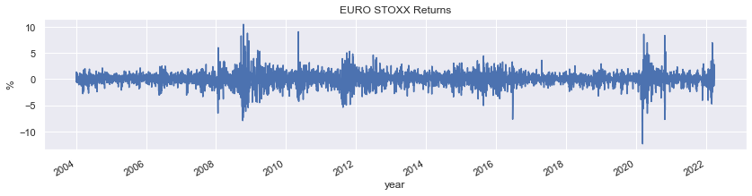
euro_stoxx_returns = 100 * euro_stoxx.pct_change().dropna()['2004':]
euro_stoxx_returns.columns = ['EURO STOXX Returns']

fig = euro_stoxx_returns.plot(figsize=(14,3), legend=False, title='EURO STOXX Returns', ylabel='%', xlabel='year')

Estimate ARCH(1)

arch1 = arch_model(y=euro_stoxx_returns, mean='constant', vol='ARCH')
arch1

Constant Mean(constant: yes, no. of exog: 0, volatility: ARCH(p: 1), distribution: Normal distribution, ID: 0x2a8f1847f70)

res = arch1.fit(update_freq=0)
print(res.summary())

Optimization terminated successfully    (Exit mode 0)
            Current function value: 7748.798771475143
            Iterations: 6
            Function evaluations: 33
            Gradient evaluations: 6
                      Constant Mean - ARCH Model Results                      
==============================================================================
Dep. Variable:     EURO STOXX Returns   R-squared:                       0.000
Mean Model:             Constant Mean   Adj. R-squared:                  0.000
Vol Model:                       ARCH   Log-Likelihood:               -7748.80
Distribution:                  Normal   AIC:                           15503.6
Method:            Maximum Likelihood   BIC:                           15523.0
                                        No. Observations:                 4749
Date:                Mon, Apr 04 2022   Df Residuals:                     4748
Time:                        17:29:15   Df Model:                            1
                                 Mean Model                                 
============================================================================
                 coef    std err          t      P>|t|      95.0% Conf. Int.
----------------------------------------------------------------------------
mu             0.0424  1.852e-02      2.288  2.212e-02 [6.082e-03,7.869e-02]
                            Volatility Model                            
========================================================================
                 coef    std err          t      P>|t|  95.0% Conf. Int.
------------------------------------------------------------------------
omega          1.2266  7.797e-02     15.731  9.201e-56 [  1.074,  1.379]
alpha[1]       0.2872  4.632e-02      6.201  5.596e-10 [  0.196,  0.378]
========================================================================

Covariance estimator: robust

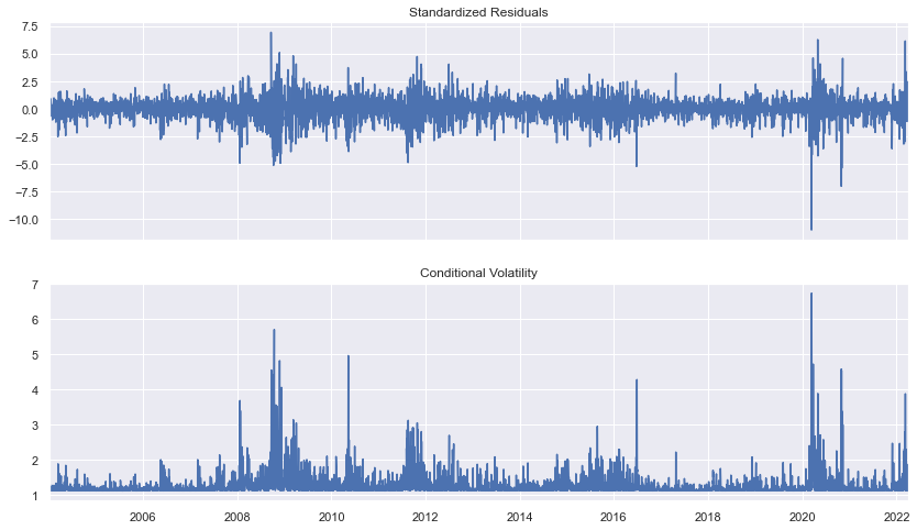
fig = res.plot()
fig.set_figheight(val=8)
fig.set_figwidth(val=14)

Forecasting

forecasts = res.forecast(reindex=False, horizon=12)

forecasts.variance

	h.01	h.02	h.03	h.04	h.05	h.06	h.07	h.08	h.09	h.10	h.11	h.12
time
2022-03-30	1.672126	1.706939	1.716939	1.719811	1.720636	1.720873	1.720941	1.720961	1.720967	1.720968	1.720969	1.720969

forecasts.mean

	h.01	h.02	h.03	h.04	h.05	h.06	h.07	h.08	h.09	h.10	h.11	h.12
time
2022-03-30	0.042386	0.042386	0.042386	0.042386	0.042386	0.042386	0.042386	0.042386	0.042386	0.042386	0.042386	0.042386

from arch.univariate import ARCH

arch7 = arch1
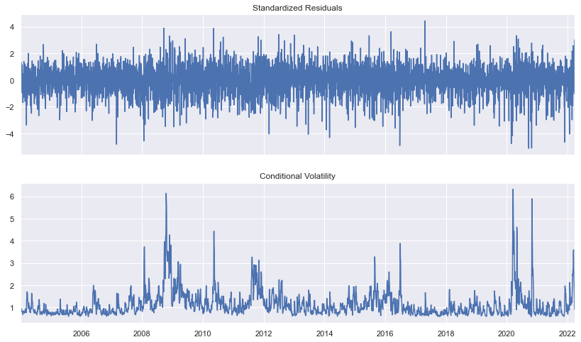
arch7.volatility = ARCH(p=7)
arch7

Constant Mean(constant: yes, no. of exog: 0, volatility: ARCH(p: 7), distribution: Normal distribution, ID: 0x2a8f1847f70)

res = arch7.fit(update_freq=0)
fig = res.plot()
fig.set_figheight(val=8)
fig.set_figwidth(val=14)

Optimization terminated successfully    (Exit mode 0)
            Current function value: 7018.71525122455
            Iterations: 19
            Function evaluations: 216
            Gradient evaluations: 19

Specifying model for the conditional mean

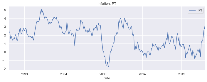
dcpi = pd.read_csv('HICP_unadj_ANR_clean.csv', index_col=0, parse_dates=True)
infl_pt = dcpi[['PT']].copy()

infl_pt.plot(figsize=(12,4), title='Inflation, PT')

<AxesSubplot:title={'center':'Inflation, PT'}, xlabel='date'>

from arch.univariate import ARX

arch_ar_model = ARX(infl_pt,
                    constant=True,
                    lags=[1, 12],
                    volatility=ARCH(p=1))

#arch_ar_model.volatility = ARCH(p=1) # to add volatility if not specified above

arch_ar_model

AR(constant: yes, lags: 1, 12, no. of exog: 0, volatility: ARCH(p: 1), distribution: Normal distribution, ID: 0x1f7a54a55d0)

$$z_t=\alpha +{\alpha }_1{z}_{t-1}+{\alpha }_{12}{z}_{t-12}+{\epsilon }_t{\epsilon }_t\sim \text{ARCH(1)}$$

res_arch_ar_model = arch_ar_model.fit(update_freq=0, disp="off")
print(res_arch_ar_model.summary())

                           AR - ARCH Model Results                            
==============================================================================
Dep. Variable:                     PT   R-squared:                       0.920
Mean Model:                        AR   Adj. R-squared:                  0.919
Vol Model:                       ARCH   Log-Likelihood:               -147.565
Distribution:                  Normal   AIC:                           305.130
Method:            Maximum Likelihood   BIC:                           323.462
                                        No. Observations:                  289
Date:                Sun, Apr 03 2022   Df Residuals:                      286
Time:                        23:43:26   Df Model:                            3
                                 Mean Model                                
===========================================================================
                 coef    std err          t      P>|t|     95.0% Conf. Int.
---------------------------------------------------------------------------
Const          0.0990  4.107e-02      2.411  1.590e-02  [1.854e-02,  0.180]
PT[1]          1.0056  1.951e-02     51.545      0.000    [  0.967,  1.044]
PT[12]        -0.0646  1.999e-02     -3.232  1.227e-03 [ -0.104,-2.544e-02]
                              Volatility Model                             
===========================================================================
                 coef    std err          t      P>|t|     95.0% Conf. Int.
---------------------------------------------------------------------------
omega          0.1288  1.829e-02      7.039  1.930e-12  [9.291e-02,  0.165]
alpha[1]       0.2623      0.142      1.853  6.389e-02 [-1.515e-02,  0.540]
===========================================================================

Covariance estimator: robust

ar_model = ARX(infl_pt,
                    constant=True,
                    lags=[1, 12])

res_ar_model = ar_model.fit(update_freq=0, disp="off")
print(res_ar_model.summary())

                     AR - Constant Variance Model Results                     
==============================================================================
Dep. Variable:                     PT   R-squared:                       0.920
Mean Model:                        AR   Adj. R-squared:                  0.920
Vol Model:          Constant Variance   Log-Likelihood:               -153.943
Distribution:                  Normal   AIC:                           315.887
Method:            Maximum Likelihood   BIC:                           330.553
                                        No. Observations:                  289
Date:                Sun, Apr 03 2022   Df Residuals:                      286
Time:                        23:43:44   Df Model:                            3
                                  Mean Model                                  
==============================================================================
                 coef    std err          t      P>|t|        95.0% Conf. Int.
------------------------------------------------------------------------------
Const          0.1315  4.353e-02      3.020  2.531e-03     [4.613e-02,  0.217]
PT[1]          0.9882  1.919e-02     51.487      0.000       [  0.951,  1.026]
PT[12]        -0.0574  1.891e-02     -3.037  2.386e-03 [-9.451e-02,-2.038e-02]
                            Volatility Model                            
========================================================================
                 coef    std err          t      P>|t|  95.0% Conf. Int.
------------------------------------------------------------------------
sigma2         0.1699  1.918e-02      8.859  8.041e-19 [  0.132,  0.207]
========================================================================

Covariance estimator: White's Heteroskedasticity Consistent Estimator

forecasts = res_arch_ar_model.forecast(reindex=False, horizon=6)
forecasts.mean

	h.1	h.2	h.3	h.4	h.5	h.6
date
2022-01-01	3.498751	3.610983	3.736772	3.82449	3.983794	4.034121

forecasts.variance

	h.1	h.2	h.3	h.4	h.5	h.6
date
2022-01-01	0.193844	0.375625	0.555719	0.736862	0.91979	1.104713

previous

Conditional Heteroskedasticity

next

Multivariate models