.ipynb .pdf

Binder

Contents

Forecasting

Time series models are (largely) models of the temporal dependence observed in time series data

• the future depends of the past

• the past is informative about the future

One motivation behind fitting models to a time series is to forecast future unobserved observations - which would not be possible without a model.

Prediction is interesting for a variety of reasons. First, it is one of the few rationalizations for time-series to be a subject of its own, divorced from economics.

Time series process $\{z_t{\}}_{t=-\mathrm{\infty }}^{\mathrm{\infty }}$

$$\begin{array}{r}{\mathit{Z}}^{\mathrm{\infty }}=\left[\begin{array}{c}⋮\\ z_{-k}\\ z_{-k+1}\\ ⋮\\ z_{-1}\\ z_0\\ z_1\\ ⋮\\ z_T\\ z_{T+1}\\ ⋮\end{array}\right]\end{array}$$

Consider $z_{T+1}$

• at time $T$ it is a random variable with some (marginal) distribution

• and a conditional distribution, given $\mathbf{z}=\{z_t{\}}_{t=1}^T$

$$p(z_{T+1}|\mathbf{z})$$

• describes all knowledge of $z_{T+1}$ given $\mathbf{z}$

• called predictive distribution

similarly for $z_{T+h}$

$$p(z_{T+h}|\mathbf{z})$$

Point forecast

• What is our best guess $z_{T+h}^f$ of $z_{T+h}$ given information availalbe as of $T$?

• Depends on how we define “best”, i.e. what the optimality criterion is

• if the goal is to minimize the expected (mean) square error

$$\mathrm{E}((z_{T+h}-z_{T+h}^f{)}^2|\mathbf{z})$$

the best point forecast is

$$\mathrm{E}(z_{T+h}|\mathbf{z})={\mathrm{E}}_T(z_{T+h})$$

• for other loss functions, the optimal forecast is another characteristics of the predictive distribution (e.g. the median)

• $p(z_{T+h}|\mathbf{z})$ and $\mathrm{E}(z_{T+h}|\mathbf{z})$ are unknown

• we use models to approximate them

Forecasting for AR(1) model

$$z_t=\alpha z_{t-1}+{\epsilon }_t$$

• at time $T$ we observe $z_1,z_2,\cdots ,z_T$ and want to forecast $z_{T+h}$

• $h=1$

$$z_{T+1}=\alpha z_T+{\epsilon }_{T+1}$$

$$\mathrm{E}(z_{T+1}|z_1,z_2,\cdots ,z_T)=\mathrm{E}(z_{T+1}|z_T)=\alpha z_T$$

why?

the information in past $z$’s is the same as information in past $\epsilon$’s, and ${\epsilon }_{T+1}$ is unpredictable

• $h=2$

$$\begin{array}{r}\begin{array}{rl}{z}_{T+2}& =\alpha z_{T+1}+{\epsilon }_{T+2}\\ & ={\alpha }^2{z}_T+\alpha {\epsilon }_{T+1}+{\epsilon }_{T+2}\end{array}\end{array}$$

$$\mathrm{E}(z_{T+2}|z_1,z_2,\cdots ,z_T)=\mathrm{E}(z_{T+2}|z_T)={\alpha }^2{z}_T$$

• for any $h>0$

$$\mathrm{E}(z_{T+h}|z_1,z_2,\cdots ,z_T)=\mathrm{E}(z_{T+h}|z_T)={\alpha }^h{z}_T$$

• as $h⟶\mathrm{\infty }$

$$\mathrm{E}(z_{T+h}|z_T)⟶0=\mathrm{E}(z_t)$$

first-order Markov process:

$$p(z_{T+1}|z_1,z_2,\cdots ,z_T)=p(z_{T+1}|z_T)$$

$z_{T+1}$ and $z_{1:T-1}$ are independent, conditional on $z_T$

higher-order Markov processes (AR§):

$z_{T+1}$ and $z_{1:T-p}$ are independent, conditional on $z_{T-p+1:T}$

Mean squared error of the forecasts (MSE)

• $h=1$

$$\begin{array}{r}\begin{array}{rl}\mathrm{E}((z_{T+1}-z_{T+1}^f{)}^2)& =\mathrm{Var}(z_{T+1}-\mathrm{E}(z_{T+1}|z_T))\\ & =\mathrm{Var}(z_{T+1}-\alpha z_T)\\ & =\mathrm{Var}\left({\epsilon }_{T+1}\right)\\ & ={\sigma }^2\end{array}\end{array}$$

• $h>1$

$$\begin{array}{r}\begin{array}{rl}\mathrm{E}((z_{T+h}-z_{T+h}^f{)}^2)& =\mathrm{Var}(z_{T+h}-{\alpha }^h{z}_T)\\ & =\mathrm{Var}({\epsilon }_{T+h}+\alpha {\epsilon }_{T+h-1}+\cdots ,+{\alpha }^{h-1}{\epsilon }_{T+1})\\ & ={\sigma }^2(1+{\alpha }^2+\cdots +{\alpha }^{2(h-1)})\end{array}\end{array}$$

• as $h⟶\mathrm{\infty }$

$$\begin{array}{r}\mathrm{E}((z_{T+h}-z_{T+h}^f{)}^2)⟶\frac{{\sigma }^2}{(1-{\alpha }^2)}=\mathrm{Var}(z_t)\end{array}$$

Forecasting for AR§ model

$$z_t={\alpha }_1{z}_{t-1}+{\alpha }_2{z}_{t-2}+\cdots +{\alpha }_p{z}_{t-p}+{\epsilon }_t$$

• $h=1$

$$z_{T+1}={\alpha }_1{z}_T+{\alpha }_2{z}_{T-1}+\cdots +{\alpha }_p{z}_{T+1-p}+{\epsilon }_{T+1}$$

$$\mathrm{E}(z_{T+1}|z_1,z_2,\cdots ,z_T)=\mathrm{E}(z_{T+1}|z_{T+1-p},\cdots ,z_{T-1},z_T)={\alpha }_1{z}_T+{\alpha }_2{z}_{T-1}+\cdots +{\alpha }_p{z}_{T+1-p}$$

for $h>1$, it is easier to use a VAR(1) representation:

$$\begin{array}{r}\underset{{\mathbf{z}}_t}{\underbrace{\left[\begin{array}{c}{z}_t\\ z_{t-1}\\ ⋮\\ z_{t-p+1}\end{array}\right]}}=\underset{\mathit{A}}{\underbrace{\left[\begin{array}{ccccc}{\alpha }_1& {\alpha }_2& \cdots & {\alpha }_{p-1}& {\alpha }_p\\ 1& 0& \cdots & 0& 0\\ ⋮& ⋮& ⋮& ⋮\\ 0& 0& \cdots & 1& 0\end{array}\right]}}\underset{{\mathbf{z}}_{t-1}}{\underbrace{\left[\begin{array}{c}{z}_{t-1}\\ z_{t-2}\\ ⋮\\ z_{t-p}\end{array}\right]}}+\underset{{\mathit{\epsilon }}_t}{\underbrace{\left[\begin{array}{c}{\epsilon }_t\\ 0\\ ⋮\\ 0\end{array}\right]}}\end{array}$$

$$\begin{array}{r}\begin{array}{rl}{\mathbf{z}}_{T+1}& =\mathit{A}{\mathbf{z}}_T+{\mathit{\epsilon }}_{T+1}\\ \mathrm{E}({\mathbf{z}}_{T+1}|{\mathbf{z}}_T)& =\mathit{A}{\mathbf{z}}_T\end{array}\end{array}$$

$$\mathrm{E}({\mathbf{z}}_{T+h}|{\mathbf{z}}_T)={\mathit{A}}^h{\mathbf{z}}_T$$

$${\mathbf{z}}_{T+h}-\mathrm{E}({\mathbf{z}}_{T+h}|{\mathbf{z}}_T)={\mathit{A}}^{h-1}{\mathit{\epsilon }}_{T+1}+{\mathit{A}}^{h+2}{\mathit{\epsilon }}_{T+2}+\cdots +{\mathit{\epsilon }}_{T+h}$$

Let $\mathbf{e}=[1,0,0,\cdots ,0{]}^{\prime }$ be a $p$ dimensional vector (first column of a $p\times p$ identity matrix). Then

$$z_{T+h}={\mathbf{e}}^{\prime }{\mathbf{z}}_{T+h}$$

and

$$\mathrm{E}(z_{T+h}|{\mathbf{z}}_T)={\mathbf{e}}^{\prime }{\mathit{A}}^h{\mathbf{z}}_T$$

$$\mathrm{E}\left[{({\mathbf{z}}_{T+h}-\mathrm{E}({\mathbf{z}}_{T+h}|{\mathbf{z}}_T))}^2\right]=({\mathit{A}}^{h-1}{\mathit{\epsilon }}_{T+1}+{\mathit{A}}^{h+2}{\mathit{\epsilon }}_{T-2}+\cdots +{\mathit{\epsilon }}_{T+h}{)}^2$$

• the MSE of the forecast:

$${\mathbf{e}}^{\prime }\mathrm{E}\left[{({\mathbf{z}}_{T+h}-\mathrm{E}({\mathbf{z}}_{T+h}|{\mathbf{z}}_T))}^2\right]\mathbf{e}={\sigma }^2(a_{h-1}^2+a_{h-2}^2+\cdots +1)$$

where $a_i={\mathbf{e}}^{\prime }{\mathit{A}}^i\mathbf{e}$

Forecasting for MA(q) and ARMA(p,q) models

MA(q)

$$z_t={\epsilon }_t+{\beta }_1{\epsilon }_{t-1}+\cdots +{\beta }_q{\epsilon }_{t-q}$$

$$z_{T+1}={\epsilon }_{T+1}+{\beta }_1{\epsilon }_T+\cdots +{\beta }_q{\epsilon }_{T-q+1}$$

$$\begin{array}{r}\begin{array}{rl}{\mathrm{E}}_T{z}_{T+1}& ={\mathrm{E}}_T{\epsilon }_{T+1}+{\beta }_1{\mathrm{E}}_T{\epsilon }_T+\cdots +{\beta }_q{\mathrm{E}}_T{\epsilon }_{T-q+1}\\ & ={\beta }_1{\mathrm{E}}_T{\epsilon }_T+\cdots +{\beta }_q{\mathrm{E}}_T{\epsilon }_{T-q+1}\end{array}\end{array}$$

$$\begin{array}{rl}{\mathrm{E}}_T{z}_{T+2}& ={\beta }_2{\mathrm{E}}_T{\epsilon }_T+\cdots +{\beta }_q{\mathrm{E}}_T{\epsilon }_{T-q+2}(h=2)\end{array}$$

$$\begin{array}{rl}{\mathrm{E}}_T{z}_{T+q}& ={\beta }_q{\mathrm{E}}_T{\epsilon }_T(h=q)\end{array}$$

• if $h>q$

$$\begin{array}{r}{\mathrm{E}}_T{z}_{T+h}=0\end{array}$$

by invertability of MA(q):

$$\begin{array}{r}\begin{array}{rl}{z}_t& =\mathit{\beta }(L){\epsilon }_t\\ {\epsilon }_t& =\frac{1}{\mathit{\beta }(L)}=\mathit{\alpha }(L)z_t\end{array}\end{array}$$

$$\begin{array}{r}\begin{array}{rl}{\mathrm{E}}_T{\epsilon }_T& ={\mathrm{E}}_T\mathit{\alpha }(L)z_T\\ & ={\mathrm{E}}_T(z_T+{\alpha }_1{z}_{T-1}+{\alpha }_2{z}_{T-2}+\cdots )\\ & =z_T+{\alpha }_1{z}_{T-1}+{\alpha }_2{z}_{T-2}+\cdots +{\alpha }_{T-1}{z}_1\end{array}\end{array}$$

import warnings
warnings.simplefilter("ignore", FutureWarning)
warnings.simplefilter("ignore", UserWarning)
from statsmodels.tools.sm_exceptions import ConvergenceWarning
warnings.simplefilter('ignore', ConvergenceWarning)

import numpy as np
from numpy.random import default_rng
from statsmodels.tsa.arima_process import arma_acovf, ArmaProcess

import statsmodels.tsa.api as smt

np.set_printoptions(precision=3, suppress=True)

getting ${\alpha }_i$ in Python

beta = np.array([.6, -.3]) # coefficients on e(t-1) and e(t-2)
ar = [1]  # coefficient on z_t
ma = np.r_[1, beta]
ma2_process = ArmaProcess(ar, ma)

ma2_process.arma2ar(100)
#statsmodels.tsa.arima_process.arma_impulse_response(ma=[1.0,], ar=[1, .6, -.3], leads=10)

array([ 1.   , -0.6  ,  0.66 , -0.576,  0.544, -0.499,  0.462, -0.427,
        0.395, -0.365,  0.338, -0.312,  0.289, -0.267,  0.247, -0.228,
        0.211, -0.195,  0.18 , -0.167,  0.154, -0.142,  0.132, -0.122,
        0.112, -0.104,  0.096, -0.089,  0.082, -0.076,  0.07 , -0.065,
        0.06 , -0.055,  0.051, -0.047,  0.044, -0.041,  0.037, -0.035,
        0.032, -0.03 ,  0.027, -0.025,  0.023, -0.022,  0.02 , -0.018,
        0.017, -0.016,  0.015, -0.014,  0.012, -0.012,  0.011, -0.01 ,
        0.009, -0.008,  0.008, -0.007,  0.007, -0.006,  0.006, -0.005,
        0.005, -0.005,  0.004, -0.004,  0.004, -0.003,  0.003, -0.003,
        0.003, -0.002,  0.002, -0.002,  0.002, -0.002,  0.002, -0.001,
        0.001, -0.001,  0.001, -0.001,  0.001, -0.001,  0.001, -0.001,
        0.001, -0.001,  0.001, -0.001,  0.001, -0.   ,  0.   , -0.   ,
        0.   , -0.   ,  0.   , -0.   ])

• the MSE of forecast:

• h = 2

$$\begin{array}{r}\begin{array}{rl}{z}_{T+2}& ={\epsilon }_{T+2}+{\beta }_1{\epsilon }_{T+1}+{\beta }_2{\epsilon }_T+\cdots +{\beta }_q{\mathrm{E}}_T{\epsilon }_{T-q+2}\\ {\mathrm{E}}_T{z}_{T+2}& ={\beta }_2{\mathrm{E}}_T{\epsilon }_T+\cdots +{\beta }_q{\mathrm{E}}_T{\epsilon }_{T-q+2}\end{array}\end{array}$$

If ${\mathrm{E}}_T{\epsilon }_T\approx {\epsilon }_T$, ${\mathrm{E}}_T{\epsilon }_{T-1}\approx {\epsilon }_{T-1}$, etc:

$$\mathrm{E}\left[{(z_{T+2}-\mathrm{E}(z_{T+2}|{\mathbf{z}}_T))}^2\right]\mathbf{e}={\sigma }^2(1+{\beta }_1^2)$$

• general $h$

$$\mathrm{E}\left[{(z_{T+h}-\mathrm{E}(z_{T+h}|{\mathbf{z}}_T))}^2\right]\mathbf{e}={\sigma }^2(1+{\beta }_1^2+{\beta }_2^2+\cdots +{\beta }_{h-1}^2)$$

ARMA(p, q)

$$\begin{array}{rl}{z}_t& ={\alpha }_1{z}_{t-1}+\cdots +{\alpha }_p{z}_{t-p}+{\epsilon }_t+{\beta }_1{\epsilon }_{t-1}+\cdots +{\beta }_q{\epsilon }_{t-q}\end{array}$$

$$z_{T+1}={\alpha }_1{z}_T+\cdots +{\alpha }_p{z}_{T-p+1}+{\epsilon }_{T+1}+{\beta }_1{\epsilon }_T+\cdots +{\beta }_q{\epsilon }_{T-q+1}$$

$$\begin{array}{rl}{\mathrm{E}}_T{z}_{T+1}& ={\alpha }_1{z}_T+\cdots +{\alpha }_p{z}_{T-p+1}+{\beta }_1{\mathrm{E}}_T{\epsilon }_T+\cdots +{\beta }_q{\mathrm{E}}_T{\epsilon }_{T-q+1}\end{array}$$

$${\mathrm{E}}_T{z}_{T+2}={\alpha }_1{\mathrm{E}}_T{z}_{T+1}+{\alpha }_2{z}_T+\cdots +{\alpha }_p{z}_{T-p+2}+{\beta }_2{\mathrm{E}}_T{\epsilon }_T+\cdots +{\beta }_q{\mathrm{E}}_T{\epsilon }_{T-q+2}$$

• obtain ${\mathrm{E}}_T{\epsilon }_T$, ${\mathrm{E}}_T{\epsilon }_{T-1}$ etc as in the MA(q) case

$$\begin{array}{r}\begin{array}{rl}\mathit{\alpha }(L)z_t& =\mathit{\beta }(L){\epsilon }_t\\ {\epsilon }_t& =\frac{\mathit{\alpha }(L)}{\mathit{\beta }(L)}{z}_t=\mathit{\psi }(L)z_t\end{array}\end{array}$$

alpha = np.array([.8])
beta = np.array([0.1])
ar = np.r_[1, -alpha] # coefficient on z(t) and z(t-1)
ma = np.r_[1, beta]  # coefficients on e(t) and e(t-1)
arma11_process = ArmaProcess(ar, ma)

arma11_process.arma2ar(8)

array([ 1.   , -0.9  ,  0.09 , -0.009,  0.001, -0.   ,  0.   , -0.   ])

Using the $MA(\mathrm{\infty })$ representation:

$$\begin{array}{r}\begin{array}{rl}\mathit{\alpha }(L)z_t& =\mathit{\beta }(L){\epsilon }_t\\ z_t& =\frac{\mathit{\beta }(L)}{\mathit{\alpha }(L)}{\epsilon }_t=\mathit{\varphi }(L){\epsilon }_t\end{array}\end{array}$$

we have $$

(3)$$\begin{array}{r}{z}_{T+h}={\epsilon }_{T+h}+{\varphi }_1{\epsilon }_{T+h-1}+{\varphi }_2{\epsilon }_{T+h-2}+\cdots +{\varphi }_h{\epsilon }_T+{\varphi }_{h+1}{\epsilon }_{T-1}+{\varphi }_{h+2}{\epsilon }_{T-2}+\cdots \end{array}$$

$$and$$

(4)$$\begin{array}{r}{\mathrm{E}}_T{z}_{T+h}={\varphi }_h{\mathrm{E}}_T{\epsilon }_T+{\varphi }_{h+1}{\mathrm{E}}_T{\epsilon }_{T-1}+{\varphi }_{h+2}{\mathrm{E}}_T{\epsilon }_{T-2}+\cdots \end{array}$$

$$

• the MSE of forecast :

$$\mathrm{E}\left[{(z_{T+h}-\mathrm{E}(z_{T+h}|{\mathbf{z}}_T))}^2\right]={\sigma }^2(1+{\varphi }_1^2+{\varphi }_2^2+\cdots +{\varphi }_{h-1}^2)$$

assuming (as for MA(q)) ${\mathrm{E}}_T{\epsilon }_T\approx {\epsilon }_T$, ${\mathrm{E}}_T{\epsilon }_{T-1}\approx {\epsilon }_{T-1}$, etc:

• in general $\mathrm{E}(z_{T+h}|\mathbf{z})$ is unknown and non-linear function of $\mathbf{z}$

Gaussian time series model

$$p(\underset{{\mathbf{z}}_1}{\underbrace{z_1,z_2,\cdots ,z_T}},\underset{{\mathbf{z}}_2}{\underbrace{z_{T+1},\cdots ,z_{T+h}}})=p({\mathbf{z}}_1,{\mathbf{z}}_2)\sim \mathcal{N}(\mathit{\mu },\mathbf{\Sigma }).$$

Then,

$$p({\mathbf{z}}_2|{\mathbf{z}}_1)=\mathcal{N}({\mathit{\mu }}_2+{\mathbf{\Sigma }}_{21}{\mathbf{\Sigma }}_{11}^{-1}({\mathbf{z}}_1-{\mathit{\mu }}_1),{\mathbf{\Sigma }}_{22}-{\mathbf{\Sigma }}_{21}{\mathbf{\Sigma }}_{11}^{-1}{\mathbf{\Sigma }}_{12})$$

• $\mathrm{E}({\mathbf{z}}_2|{\mathbf{z}}_1)={\mathit{\mu }}_2+{\mathbf{\Sigma }}_{21}{\mathbf{\Sigma }}_{11}^{-1}({\mathbf{z}}_1-{\mathit{\mu }}_1)$ optimal forecast

• $\mathrm{cov}({\mathbf{z}}_2|{\mathbf{z}}_1)={\mathbf{\Sigma }}_{22}-{\mathbf{\Sigma }}_{21}{\mathbf{\Sigma }}_{11}^{-1}{\mathbf{\Sigma }}_{12}$ MSE of the optimal forecast

• we can restrict “best” to apply to linear functions only: best linear predictor of $z_{T+h}$ given $\mathbf{z}$

$$\begin{array}{}\text{(1)}& z_{T+h}^f={\beta }_0+{\beta }_1^{\prime }\mathbf{z}\end{array}$$

• if the loss is the MSE, the best linear predictor is (1) with

$$\begin{array}{r}\begin{array}{rl}{\beta }_0& =\mathrm{E}{z}_{T+h}-\mathrm{Cov}(z_{T+h},\mathbf{z})\mathrm{Cov}(\mathbf{z},\mathbf{z}{)}^{-1}\mathrm{E}\mathbf{z}\\ {\beta }_1& =\mathrm{Cov}(z_{T+h},\mathbf{z})\mathrm{Cov}(\mathbf{z},\mathbf{z}{)}^{-1}\end{array}\end{array}$$

Prediction operator

the best linear prediction of random variable $y$ given a random vector $\mathbf{z}$

$$\begin{array}{r}\begin{array}{rl}\mathrm{P}(y|\mathbf{z})& ={\mu }_y+{\varphi }^{\prime }(\mathbf{z}-{\mu }_{\mathbf{z}})\\ \\ \text{with}\\ \\ {\varphi }^{\prime }& =\mathrm{cov}(y,\mathbf{z}{)}^{\prime }\mathrm{cov}(\mathbf{z},\mathbf{z}{)}^{-1}\end{array}\end{array}$$

• has lowest MSE loss

the MSE of $\mathrm{P}(y|\mathbf{z})$:

$$\mathrm{E}\left[{(y-\mathrm{P}(y|\mathbf{z}))}^2\right]=\mathrm{var}(y)-\mathrm{cov}(y,\mathbf{z}{)}^{\prime }\mathrm{cov}(\mathbf{z},\mathbf{z}{)}^{-1}\mathrm{cov}(y,\mathbf{z})$$

properties of $\mathrm{P}(y|\mathbf{z})$ :

• $\mathrm{E}(y-\mathrm{P}(y|\mathbf{z}))=0$

• $\mathrm{E}((y-\mathrm{P}(y|\mathbf{z}))\mathbf{z})=0$

• $\mathrm{P}(z_i|\mathbf{z}))=z_i$

• $\mathrm{P}(y|\mathbf{z}))=\mathrm{E}y$, if $\mathrm{cov}(y,\mathbf{z})=0$

ARMA forecasting in Python

import pandas as pd
import matplotlib.pyplot as plt
from statsmodels.tsa.arima.model import ARIMA
from numpy.random import default_rng

• generate data from ARMA(1,1)

gen = default_rng(100)
T=700
z = arma11_process.generate_sample(T, distrvs=gen.normal)

• estimate

arma_model = ARIMA(z, order=(1, 0, 1), trend="n")
arma_results = arma_model.fit()
print(arma_results.summary())

                               SARIMAX Results                                
==============================================================================
Dep. Variable:                      y   No. Observations:                  700
Model:                 ARIMA(1, 0, 1)   Log Likelihood                -998.176
Date:                Mon, 21 Mar 2022   AIC                           2002.351
Time:                        10:22:36   BIC                           2016.005
Sample:                             0   HQIC                          2007.629
                                - 700                                         
Covariance Type:                  opg                                         
==============================================================================
                 coef    std err          z      P>|z|      [0.025      0.975]
------------------------------------------------------------------------------
ar.L1          0.8075      0.027     29.733      0.000       0.754       0.861
ma.L1          0.0199      0.047      0.423      0.672      -0.072       0.112
sigma2         1.0126      0.058     17.456      0.000       0.899       1.126
===================================================================================
Ljung-Box (L1) (Q):                   0.00   Jarque-Bera (JB):                 2.05
Prob(Q):                              0.98   Prob(JB):                         0.36
Heteroskedasticity (H):               1.06   Skew:                             0.06
Prob(H) (two-sided):                  0.66   Kurtosis:                         2.76
===================================================================================

Warnings:
[1] Covariance matrix calculated using the outer product of gradients (complex-step).

• forecast the next 5 values

arma_results.forecast(steps=5)

array([-0.816, -0.659, -0.532, -0.43 , -0.347])

• get forecasts and CI

fcast_res = arma_results.get_forecast(steps=5,)
fcast_res.summary_frame()

y	mean	mean_se	mean_ci_lower	mean_ci_upper
0	-0.815737	1.006267	-2.787985	1.156510
1	-0.658719	1.306041	-3.218512	1.901073
2	-0.531925	1.468926	-3.410966	2.347116
3	-0.429537	1.566040	-3.498920	2.639846
4	-0.346857	1.626246	-3.534241	2.840527

• working with dates

data = pd.DataFrame(z, index=pd.date_range(start='1964', freq='M', periods=T), columns=['z'])
data.tail() 

	z
2021-12-31	-1.983945
2022-01-31	-3.883839
2022-02-28	-2.971514
2022-03-31	-2.339958
2022-04-30	-1.031274

arma_model = ARIMA(data, order=(1, 0, 1), trend="n")
arma_results = arma_model.fit()

fcast_res = arma_results.get_forecast(steps=24)
fcast = fcast_res.summary_frame()
fcast.head()

z	mean	mean_se	mean_ci_lower	mean_ci_upper
2022-05-31	-0.815737	1.006267	-2.787985	1.156510
2022-06-30	-0.658719	1.306041	-3.218512	1.901073
2022-07-31	-0.531925	1.468926	-3.410966	2.347116
2022-08-31	-0.429537	1.566040	-3.498920	2.639846
2022-09-30	-0.346857	1.626246	-3.534241	2.840527

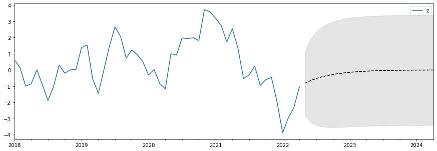
• plot forecasts

fig, ax = plt.subplots(figsize=(15, 5))

# Plot the data (here we are subsetting it to get a better look at the forecasts)
data.loc['2018':].plot(ax=ax)
# Construct the forecasts
fcast['mean'].plot(ax=ax, style='k--')
ax.fill_between(fcast.index, fcast['mean_ci_lower'], fcast['mean_ci_upper'], color='k', alpha=0.1);
 

In-sample forecast evaluation

use

$$\frac{1}{T}\sum _{t=0}^{T-1}{(z_{t+1}-{\hat{z}}_{t+1}^f)}^2$$

as an estimate of the MSE

$$\mathrm{E}((z_{t+1}-z_{t+1}^f{)}^2)$$

data['forecast'] = arma_results.forecasts.flatten()
data['forecast errors'] = arma_results.forecasts_error.flatten()

data.tail()

	z	forecast	forecast errors
2021-12-31	-1.983945	-0.373014	-1.610931
2022-01-31	-3.883839	-1.634070	-2.249770
2022-02-28	-2.971514	-3.180953	0.209439
2022-03-31	-2.339958	-2.395378	0.055420
2022-04-30	-1.031274	-1.888448	0.857174

(arma_results.forecasts_error**2).sum()/T

1.0138467224702907

arma_results.mse

1.0138467224702907

In-sample forecasts are based on model estimated using the full sample

• in AR(1) model

$${\hat{z}}_{t+1}^f=\hat{\alpha }{z}_t$$

introduces information from the future relative to the time ($t<T$) when forecasts are produced

Out-of-sample (OOS) forecast evaluation

parameter estimates of the forecasting model use only information available at the time when the forecast is computed

• fit the model on a training sample $z_1,\cdots ,z_t$ for some $t=t_0<T$

• produce forecast ${\hat{z}}_{t+1}^f$ from the end of that sample

• compare to true value $z_{t+1}$

• expand the sample to include the next observation, and repeat until $t=T-1$

The OOS estimate of MSE

$$\frac{1}{T-t_0}\sum _{t=t_0-1}^{T-1}{(z_{t+1}-{\hat{z}}_{t+1}^f)}^2$$

data = data[['z']]

# Setup forecasts
nforecasts = 1
forecasts = {}

# Get the number of initial training observations
nobs = len(data)
n_init_training = int(nobs * 0.8)

# Create model for initial training sample, fit parameters
init_training_endog = data.iloc[:n_init_training]
mod = ARIMA(init_training_endog, order=(1, 0, 1), trend="n")
res = mod.fit()

# Save initial forecast
forecasts[init_training_endog.index[-1]] = res.forecast(steps=nforecasts)

# Step through the rest of the sample
for t in range(n_init_training, nobs-1):
    # Update the results by appending the next observation
    updated_data = data.iloc[t:t+1]
    res = res.append(updated_data, refit=True)

    # Save the new set of forecasts
    forecasts[updated_data.index[0]] = res.forecast(steps=nforecasts)

# Combine all forecasts into a dataframe
forecasts = pd.concat(forecasts, axis=1)

forecasts.iloc[:5, :5]

	2010-08-31	2010-09-30	2010-10-31	2010-11-30	2010-12-31
2010-09-30	1.632432	NaN	NaN	NaN	NaN
2010-10-31	NaN	0.928112	NaN	NaN	NaN
2010-11-30	NaN	NaN	0.127096	NaN	NaN
2010-12-31	NaN	NaN	NaN	1.271923	NaN
2011-01-31	NaN	NaN	NaN	NaN	0.60945

forecasts.iloc[-5:, -5:]

	2021-11-30	2021-12-31	2022-01-31	2022-02-28	2022-03-31
2021-12-31	-0.373446	NaN	NaN	NaN	NaN
2022-01-31	NaN	-1.62698	NaN	NaN	NaN
2022-02-28	NaN	NaN	-3.185304	NaN	NaN
2022-03-31	NaN	NaN	NaN	-2.400559	NaN
2022-04-30	NaN	NaN	NaN	NaN	-1.891933

# Construct the forecast errors
forecast_errors = {}
for c in forecasts.columns:
    forecast_errors[c] = data.iloc[n_init_training:, 0] - forecasts.loc[:,c]
    
forecast_errors = pd.DataFrame.from_dict(forecast_errors)    

def flatten(column):
    return column.dropna().reset_index(drop=True)

flattened = forecast_errors.apply(flatten)
flattened.index = (flattened.index + 1).rename('horizon')
flattened.T.head()

horizon	1
2010-08-31	-0.496213
2010-09-30	-0.757934
2010-10-31	1.392945
2010-11-30	-0.523532
2010-12-31	-0.075812

forecast_errors = flattened.T.dropna().values.flatten()

# Compute the root mean square error
rmse = (forecast_errors**2).mean()**0.5

print(rmse)

1.0117784839655213

previous

ARMA models

next

Non-stationarity