.ipynb .pdf

Binder

Contents

Appilcations of state space models

ARMA(p,q) models

Example

MA(1)

$$z_t={\epsilon }_t+\beta {\epsilon }_{t-1}$$

State space form

$$\begin{array}{r}\begin{array}{rl}\left[\begin{array}{c}{\epsilon }_t\\ {\epsilon }_{t-1}\end{array}\right]& =\left[\begin{array}{cc}0& 0\\ 1& 0\end{array}\right]\left[\begin{array}{c}{\epsilon }_{t-1}\\ {\epsilon }_{t-2}\end{array}\right]+\left[\begin{array}{c}{\epsilon }_t\\ 0\end{array}\right]\\ \\ z_t& =\left[\begin{array}{c}1\beta \end{array}\right]\left[\begin{array}{c}{\epsilon }_t\\ {\epsilon }_{t-1}\end{array}\right]\end{array}\end{array}$$

Example ARMA(2,1)

$$z_t={\alpha }_1{z}_{t-1}+{\alpha }_2{z}_{t-2}+{\epsilon }_t+\beta {\epsilon }_{t-1}$$

State space form

$$\begin{array}{r}\begin{array}{rl}\left[\begin{array}{c}{x}_{1,t}\\ x_{2,t}\end{array}\right]& =\left[\begin{array}{cc}{\alpha }_1& {\alpha }_2\\ 1& 0\end{array}\right]\left[\begin{array}{c}{x}_{1,t-1}\\ x_{2,t-1}\end{array}\right]+\left[\begin{array}{c}{\epsilon }_t\\ 0\end{array}\right]\\ z_t& =\left[\begin{array}{c}1\beta \end{array}\right]\left[\begin{array}{c}{x}_{1,t}\\ x_{2,t}\end{array}\right]\end{array}\end{array}$$

$$\begin{array}{r}\begin{array}{rl}{z}_t& =\beta (L)x_{1,t}\\ x_{1,t}& =\alpha (L{)}^{-1}{w}_t\\ \alpha (L)z_t& =\beta (L)w_t\end{array}\end{array}$$

Generalizes to ARMA(p,q)

Unobserved-components models

Example

$$\begin{array}{r}\begin{array}{rl}{z}_t& ={\tau }_t+c_t\\ {\tau }_t& ={\tau }_{t-1}+{\eta }_t\\ c_t& ={\varphi }_1{c}_{t-1}+{\varphi }_2{c}_{t-2}+{\epsilon }_t\end{array}\end{array}$$

State space form

$$\mathrm{\Delta }{z}_t={\eta }_t+\mathrm{\Delta }{c}_t$$

$$\begin{array}{r}\begin{array}{rl}\left[\begin{array}{c}{c}_t\\ c_{t-1}\end{array}\right]& =\left[\begin{array}{cc}{\varphi }_1& {\varphi }_2\\ 1& 0\end{array}\right]\left[\begin{array}{c}{c}_{t-1}\\ c_{t-2}\end{array}\right]+\left[\begin{array}{c}{\epsilon }_t\\ 0\end{array}\right]\\ \\ \mathrm{\Delta }{z}_t& =\left[\begin{array}{c}1-1\end{array}\right]\left[\begin{array}{c}{c}_t\\ c_{t-1}\end{array}\right]+{\eta }_t\\ \end{array}\end{array}$$

$$\begin{array}{r}\begin{array}{rl}{z}_t& ={\tau }_t+c_t\\ {\tau }_t& ={\tau }_{t-1}+{\eta }_t\\ c_t& ={\varphi }_1{c}_{t-1}+{\varphi }_2{c}_{t-2}+{\epsilon }_t\end{array}\end{array}$$

State space form for the level of $z_t$

$$\begin{array}{r}\begin{array}{rl}\left[\begin{array}{c}{\tau }_t\\ c_t\\ c_{t-1}\end{array}\right]& =\left[\begin{array}{ccc}1& 0& 0\\ 0& {\varphi }_1& {\varphi }_2\\ 0& 1& 0\end{array}\right]\left[\begin{array}{c}{\tau }_{t-1}\\ c_{t-1}\\ c_{t-2}\end{array}\right]+\left[\begin{array}{c}{\eta }_t\\ {\epsilon }_t\end{array}\right]\\ \\ z_t& =\left[\begin{array}{c}110\end{array}\right]\left[\begin{array}{c}{\tau }_t\\ c_t\\ c_{t-1}\end{array}\right]\\ \end{array}\end{array}$$

Unobserved-components models in Statsmodels

Time-varying parameters

$$\begin{array}{r}\begin{array}{rl}{z}_t& =x_t{\beta }_t+{\epsilon }_t\\ {\beta }_t& ={\beta }_{t-1}+{\eta }_t\end{array}\end{array}$$

Dynamic Factor models

Example

$$\begin{array}{r}\begin{array}{rl}& \text{observed variables}\\ z_{1,t}& ={\lambda }_1{f}_t+u_{1,t}\\ z_{2,t}& ={\lambda }_1{f}_t+u_{2,t}\\ \\ & \text{common factor}\\ f_t& =\alpha f_{t-1}+{\eta }_t\\ \\ & \text{idiosyncratic components}\\ u_{1,t}& ={\varphi }_1{u}_{1,t-1}+{\epsilon }_{1,t}\\ u_{2,t}& ={\varphi }_2{u}_{2,t-1}+{\epsilon }_{2,t}\end{array}\end{array}$$

State Space form

$$\begin{array}{r}\begin{array}{rl}\left[\begin{array}{c}{f}_t\\ u_{1,t}\\ u_{2,t}\end{array}\right]& =\left[\begin{array}{ccc}\alpha & 0& 0\\ 0& {\varphi }_1& 0\\ 0& 0& {\varphi }_2\end{array}\right]\left[\begin{array}{c}{f}_{t-1}\\ u_{1,t-1}\\ u_{2,t-1}\end{array}\right]+\left[\begin{array}{c}{\eta }_t\\ {\epsilon }_{1,t}\\ {\epsilon }_{2,t}\end{array}\right]\\ \\ \left[\begin{array}{c}{z}_{1,t}\\ z_{2,t}\end{array}\right]& =\left[\begin{array}{ccc}{\lambda }_1& 1& 0\\ {\lambda }_2& 0& 1\end{array}\right]\left[\begin{array}{c}{f}_t\\ u_{1,t}\\ u_{2,t}\end{array}\right]\end{array}\end{array}$$

• can be extended to multiple factors evolving as VAR(q)

• and more general AR processes for the idiosyncratic components

DFM are a parsimoneous alternative to VARs with many series

Dynamic factor models in Statsmodels

related common trend model

$$\begin{array}{r}\begin{array}{rl}& \text{observed variables}\\ z_{1,t}& =f_t+u_{1,t}\\ z_{2,t}& =f_t+u_{2,t}\\ \\ & \text{common trend}\\ f_t& =f_{t-1}+{\eta }_t\\ \\ & \text{stationary terms}\\ u_{1,t}& ={\varphi }_1{u}_{1,t-1}+{\epsilon }_{1,t}\\ u_{2,t}& ={\varphi }_2{u}_{2,t-1}+{\epsilon }_{2,t}\end{array}\end{array}$$

State Space form

$$\begin{array}{r}\begin{array}{rl}\left[\begin{array}{c}{f}_t\\ u_{1,t}\\ u_{2,t}\end{array}\right]& =\left[\begin{array}{ccc}1& 0& 0\\ 0& {\varphi }_1& 0\\ 0& 0& {\varphi }_2\end{array}\right]\left[\begin{array}{c}{f}_{t-1}\\ u_{1,t-1}\\ u_{2,t-1}\end{array}\right]+\left[\begin{array}{c}{\eta }_t\\ {\epsilon }_{1,t}\\ {\epsilon }_{2,t}\end{array}\right]\\ \\ \left[\begin{array}{c}{z}_{1,t}\\ z_{2,t}\end{array}\right]& =\left[\begin{array}{ccc}{\lambda }_1& 1& 0\\ {\lambda }_2& 0& 1\end{array}\right]\left[\begin{array}{c}{f}_t\\ u_{1,t}\\ u_{2,t}\end{array}\right]\end{array}\end{array}$$

• $z_{1,t}$ and $z_{2,t}$ share a common stochastic trend - cointegrated

• the stationary terms can have more complicated dynamics, and may be correlated (e.g VAR instead of AR processes)

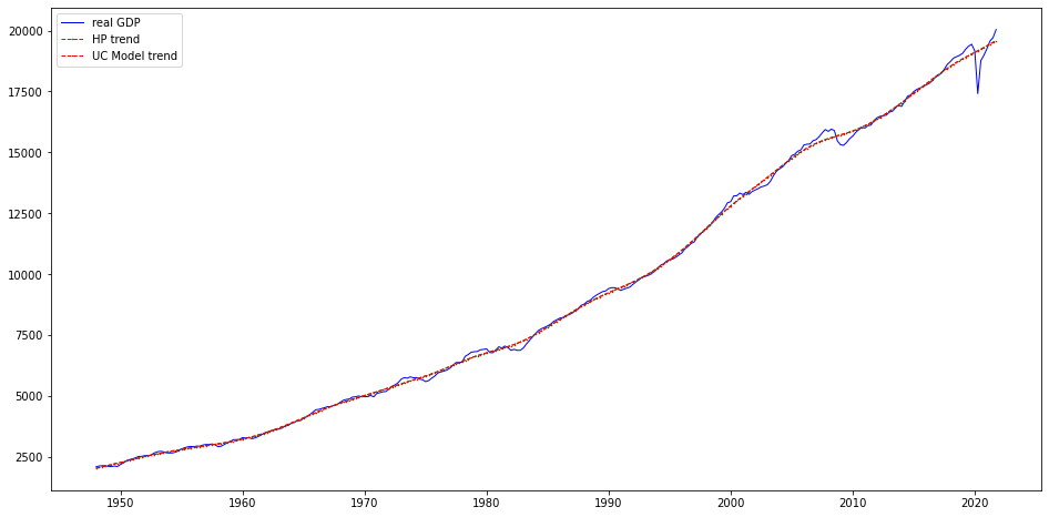
The Hodrick-Prescott filter

$$\begin{array}{r}\begin{array}{rl}{z}_t& ={\tau }_t+c_t\\ \\ \underset{{\tau }_t}{\min }(\sum _{t=1}^T(z_t-{\tau }_t{)}^2& +\lambda \sum _{t=1}^T({\tau }_t-2{\tau }_{t-1}+{\tau }_{t-2}{)}^2)\end{array}\end{array}$$

Unobserved components model

$$\begin{array}{r}\begin{array}{rl}{z}_t& ={\tau }_t+c_t\\ {\tau }_t& ={\tau }_{t-1}+{\beta }_{t-1}+{\eta }_t\\ {\beta }_t& ={\beta }_{t-1}+{\epsilon }_t\end{array}\end{array}$$

State space form

$$\begin{array}{r}\begin{array}{rl}\left[\begin{array}{c}{\tau }_t\\ {\beta }_t\end{array}\right]& =\left[\begin{array}{cc}1& 1\\ 0& 1\end{array}\right]\left[\begin{array}{c}{\tau }_{t-1}\\ {\beta }_{t-1}\end{array}\right]+\left[\begin{array}{c}{\eta }_t\\ {\epsilon }_t\end{array}\right]\\ \\ z_t& =\left[\begin{array}{c}10\end{array}\right]\left[\begin{array}{c}{\tau }_t\\ {\beta }_t\end{array}\right]+c_t\\ \end{array}\end{array}$$

$$c_t\sim \mathcal{N}(0,{\sigma }_c^2),{\epsilon }_t\sim \mathcal{N}(0,{\sigma }_{\epsilon }^2),{\eta }_t\sim \mathcal{N}(0,{\sigma }_{\eta }^2)$$

$$\text{HP-filter restrictions: }{\sigma }_{\eta }^2=0,\frac{{\sigma }_c^2}{{\sigma }_{\epsilon }^2}=\lambda$$

• no parameters are estimated

• the parameters can be estimated and the restrictions tested

Why You Should Never Use the Hodrick-Prescott Filter

import statsmodels.tsa.api as tsa
from pathlib import Path
import pandas as pd
import matplotlib.pyplot as plt

from fredapi import Fred
fred = Fred(api_key=your_api_key)
start = '1948-01'
end = '2022-01'
df_raw = fred.get_series('GNPC96',  observation_start=start, observation_end=end)
df_raw.index.freq = 'QS'
df_raw.name = 'gdpc1'
df_raw = df_raw.to_frame()
df_raw.head()

	gdpc1
1948-01-01	2102.422
1948-04-01	2137.588
1948-07-01	2149.832
1948-10-01	2152.212
1949-01-01	2122.155

hp_cycle, hp_trend = tsa.filters.hpfilter(df_raw[['gdpc1']], lamb=1600)

mod = tsa.UnobservedComponents(df_raw[['gdpc1']], 'lltrend')
res = mod.smooth([1., 0, 1. / 1600]) # 'sigma2.irregular', 'sigma2.level', 'sigma2.trend'
#print(res.summary())

ucm_trend = pd.Series(res.level.smoothed, index=df_raw[['gdpc1']].index)
fig, ax = plt.subplots(figsize=(16, 8))

ax.plot(df_raw[['gdpc1']], label='real GDP', color='blue', linestyle='solid', linewidth=1)
ax.plot(hp_trend, label='HP trend', color='green', marker='o', linestyle='dashed', linewidth=1, markersize=.5)
ax.plot(ucm_trend, label='UC Model trend', color='red', marker='+', linestyle='dashed', linewidth=1, markersize=.5)
ax.legend();

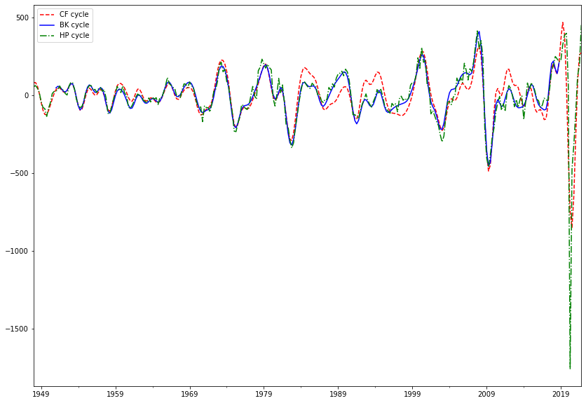
Frequency-domain filters

• time series can be thought of as the sum of periodic functions (fluctuations)

  • frequency domain, spectral analysis of time series

• business cycle components of time series correspond a subset of those fluctuations

  • those with period greater than 1.5 (or 2) years and less than 8 years

  • faster (shorter period) or slower (longer period) fluctuations are interpreted as being outside the business cycle

    • low, business cycle, high frequencies

• frequency-domain filters aim to extract the business cycle components

  • Baxter-King, Christiano-Fitzgerald

periodic functions?

• $\cos (x)=\cos (x+2k\pi ),k=1,2,\cdots$

• $\sin (x)=\sin (x+2k\pi ),k=1,2,\cdots$

• as function of time: $\cos (t\omega ),t=t_1,t_2,\cdots$

• periodicity means that

$$\begin{array}{r}\begin{array}{rl}\cos (\omega t_1)& =\cos (\omega t_h)\\ \\ \omega t_h& =\omega t_1+2\pi \\ \\ t_h-t_1& =\frac{2\pi }{\omega }\end{array}\end{array}$$

• $\omega$ is the frequency, $t_h-t_1$ is the period

• a time series $z_t$ can be represented as a sum (integral) of

$$\begin{array}{r}\end{array}$$

$$\begin{array}{r}a(\omega )\cos (\omega t)+b(\omega )\sin (\omega t),\omega \in (0,\pi )\end{array}$$

• business cycle component contains only those components with period between 1.5 and 8 years

  • with quarterly data: $\frac{2\pi }{32}\le \omega \le \frac{2\pi }{6}$

  • with monthly data: $\frac{2\pi }{96}\le \omega \le \frac{2\pi }{18}$

• band-pass filter: keep only a subset (band) of $\omega$’s in $(0,\pi )$

• both Baxter-King and Christiano-Fitzgerald filters are computed as weighted moving averages of the series, the difference is in what the weights are

  • symmetric (BK) vs asymmetric (CF) weights

  • truncated on both ends (BK) vs using the full sample (CF)

bk_cycle = tsa.filters.bkfilter(df_raw[['gdpc1']])
cf_cycle, _ = tsa.filters.cffilter(df_raw[['gdpc1']])

cf_cycle.name = 'CF cycle'
bk_cycle.columns = ['BK cycle']
hp_cycle.name = 'HP cycle'

fig = plt.figure(figsize=(14, 10))
ax = fig.add_subplot(111)
cf_cycle.plot(ax=ax, style=["r--", ], legend=True)
bk_cycle.plot(ax=ax, style=["b-", ], legend=True)
hp_cycle.plot(ax=ax, style=["g-.", ], legend=True)

<AxesSubplot:>

Frequency domain log-likelihood

Whittle log-likelihood

$$\begin{array}{r}\begin{array}{rl}\ell (\mathit{\theta }|\mathbf{z})& =\sum _{\omega }{\ell }_{\omega }(\mathit{\theta }|\mathbf{z}),\omega \in (\frac{2\pi j}{T},j=1,2,\cdots ,T)\\ \\ {\ell }_{\omega }(\mathit{\theta }|\mathbf{z})=-\ln (2\pi )& -\frac{1}{2}\ln (det(f_{\mathbf{z}}(\omega ,\mathit{\theta })))-\frac{1}{2}\mathrm{tr}(f_{\mathbf{z}}(\omega ,\mathit{\theta }{)}^{-1}I(\omega ,\mathbf{z}))\end{array}\end{array}$$

• $f_{\mathbf{z}}(\omega ,\mathit{\theta })$ is the model-implied spectral density of $\mathbf{z}$ at $\omega$

• $I(\omega ,\mathbf{z})$ is the periodogram of $\mathbf{z}$ at $\omega$

• it is like a Gaussian log-likelihood for independent observations

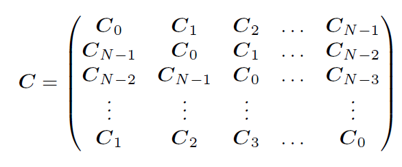
• can be derived by approximating the covariance matrix of $\mathbf{z}$ by a block circulant matrix, which can be diagonalized using DFT

  $${\mathbf{z}}^{\prime }{\mathbf{\Sigma }}^{-1}(\theta )\mathbf{z}\approx \mathrm{tr}({\mathbf{z}}^{\prime }{\mathbf{C}}^{-1}(\theta )\mathbf{z})=\mathrm{tr}({\mathbf{z}}^{\prime }{V}^{\prime }{\mathbf{F}}^{-1}(\theta )V\mathbf{z})=\sum _{\omega }\mathrm{tr}(f(\omega ,\mathit{\theta }{)}^{-1}I(\omega ,\mathbf{z}))$$

Block circulant matrix

The Whittle log-likelihood can be used as

• an alternative to the Kalman filter

• a way to estimate a model using only a subset of frequencies, e.g. BC frequencies

  • QUANTIFYING CONFIDENCE (2018) by Angeletos, Collard, Dellas

previous

State space models

next

Other topics