.ipynb .pdf

Binder

Contents

Introduction to AR and MA models

Time series models

• aim to capture complex temporal dependence

• build by combining processes with simple dependence structure - innovations

Innovations

$$\mathit{\epsilon }=\{{\epsilon }_t\},\mathrm{E}({\epsilon }_t)=0,\mathrm{var}({\epsilon }_t)={\sigma }^2$$

• white noise

• martingale difference

• iid

Linear time series models

• The time series $\mathbf{z}$ and the innovation $\mathit{\epsilon }$ are linearly related

$$\mathit{z}=\mathit{A}\mathit{\epsilon }$$

• or more generally, the transformation $\mathit{\epsilon }\to \mathbf{z}$ is affine

$$\mathit{z}=\mathit{\mu }+\mathit{A}\mathit{\epsilon }$$

• with Gaussian innovations $p(\mathit{\epsilon })\sim \mathcal{N}(\mathbf{0},{\sigma }^2\mathbf{I})$

$$\mathit{z}=\mathit{\mu }+\mathit{A}\mathit{\epsilon }\sim \mathcal{N}(\mathit{\mu },\mathbf{\Sigma }),\mathbf{\Sigma }={\sigma }^2\mathit{A}{\mathit{A}}^{\prime }$$

Moving Average (MA) models

$$z_t=\sum _{i=0}^q{\theta }_i{\epsilon }_{t-i}$$

MA(1)

$$z_t={\epsilon }_t+\theta {\epsilon }_{t-1}$$

$$\begin{array}{r}\begin{array}{rl}{z}_1& =\theta {\epsilon }_0+{\epsilon }_1\\ z_2& =\theta {\epsilon }_1+{\epsilon }_2\\ & ⋮\\ z_T& =\theta {\epsilon }_{T-1}+{\epsilon }_T\end{array}\end{array}$$

$$\begin{array}{r}\underset{\mathbf{z}}{\underbrace{\left[\begin{array}{c}{z}_1\\ z_2\\ z_3\\ z_4\\ ⋮\\ z_T\end{array}\right]}}=\underset{\mathit{A}}{\underbrace{\left[\begin{array}{cccccccc}\theta & 1& 0& 0& \cdots & 0& 0& 0\\ 0& \theta & 1& 0& \cdots & 0& 0& 0\\ 0& 0& \theta & 1& \cdots & 0& 0& 0\\ 0& 0& 0& \theta & \cdots & 0& 0& 0\\ ⋮& ⋮& ⋮& ⋮& \cdots & ⋮& ⋮& ⋮\\ 0& 0& 0& 0& \cdots & 0& \theta & 1\end{array}\right]}}\underset{\mathit{\epsilon }}{\underbrace{\left[\begin{array}{c}{\epsilon }_0\\ {\epsilon }_1\\ {\epsilon }_2\\ {\epsilon }_3\\ {\epsilon }_4\\ ⋮\\ {\epsilon }_T\end{array}\right]}}\end{array}$$

Stationarity conditions

• constant mean?

$$\mathrm{E}{z}_t=0$$

• constant variance?

$$\gamma (0)={\sigma }^2(1+{\theta }^2)$$

• constant covariances?

for lag $h=1$

$$\begin{array}{r}\begin{array}{rl}\gamma (1)=\mathrm{cov}(z_t,z_{t-1})& =\mathrm{E}(z_t{z}_{t-1})=\mathrm{E}(({\epsilon }_t+\theta {\epsilon }_{t-1})({\epsilon }_{t-1}+\theta {\epsilon }_{t-2}))\\ & =\mathrm{E}({\epsilon }_t{\epsilon }_{t-1}+\theta {\epsilon }_{t-1}^2+\theta {\epsilon }_t{\epsilon }_{t-2}+{\theta }^2{\epsilon }_{t-1}{\epsilon }_{t-2})\\ & =\theta {\sigma }^2\end{array}\end{array}$$

for lag $h\ge 2$

$$\begin{array}{r}\begin{array}{rl}\gamma (h)=\mathrm{cov}(z_t,z_{t-h})& =\mathrm{E}(({\epsilon }_t+\theta {\epsilon }_{t-1})({\epsilon }_{t-h}+\theta {\epsilon }_{t-h-1}))\\ & =0\end{array}\end{array}$$

import warnings
warnings.simplefilter("ignore", FutureWarning)

import matplotlib.pyplot as plt
import numpy as np
from statsmodels.tsa.arima_process import arma_acovf
from scipy.linalg import toeplitz

from matplotlib import rc
rc('font',**{'family':'serif','serif':['Palatino']})
rc('text', usetex=True)


plt.rcParams.update({'ytick.left' : True,
                     "xtick.bottom" : True,
                     "ytick.major.size": 0,
                     "ytick.major.width": 0,
                     "xtick.major.size": 0,
                     "xtick.major.width": 0,
                     "ytick.direction": 'in',
                     "xtick.direction": 'in',
                     'ytick.major.right': False,
                     'xtick.major.top': True,
                     'xtick.top': True,
                     'ytick.right': True,
                     'ytick.labelsize': 18,
                     'xtick.labelsize': 18
                    })

np.random.seed(12345)

def correlation_from_covariance(covariance):
    v = np.sqrt(np.diag(covariance))
    outer_v = np.outer(v, v)
    correlation = covariance / outer_v
    correlation[covariance == 0] = 0
    return correlation


def show_covariance(cov_mat, process_name):
    K = cov_mat.shape[0]
    
    fig, ax = plt.subplots(nrows=1, ncols=1, figsize=(20,8))

    
    c = ax.imshow(cov_mat,
                       cmap="magma_r",
                      )
    
    #c = ax.pcolormesh(Sigma, edgecolors='k', linewidth=.01, cmap='inferno_r')
    #ax = plt.gca()
    #ax.set_aspect('equal')
    #ax.invert_yaxis()


    plt.colorbar(c);


    ax.set_xticks(range(0,K))
    ax.set_xticklabels(range(1, K+1));
    ax.set_yticks(range(0,K))
    ax.set_yticklabels(range(1, K+1));  
    ax.set_title(f'Covariance {process_name}', fontsize=24)

    plt.subplots_adjust(wspace=-0.7)

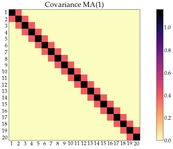
n_obs = 20
arparams = np.array([0])
maparams = np.array([.4])
ar = np.r_[1, -arparams] # add zero-lag and negate
ma = np.r_[1, maparams] # add zero-lag
sigma2=np.array([1])

acov_ma1 = arma_acovf(ar=ar, ma=ma, nobs=n_obs, sigma2=sigma2)

Sigma_ma1 = toeplitz(acov_ma1)

corr_ma1 = correlation_from_covariance(Sigma_ma1)

show_covariance(cov_mat=Sigma_ma1, process_name='MA(1)')

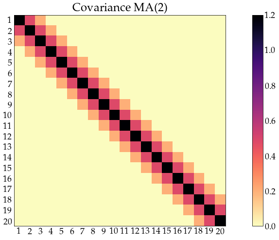
n_obs = 20
arparams = np.array([0])
maparams = np.array([.4, .2])
ar = np.r_[1, -arparams] # add zero-lag and negate
ma = np.r_[1, maparams] # add zero-lag
sigma2=np.array([1])

acov_ma2 = arma_acovf(ar=ar, ma=ma, nobs=n_obs, sigma2=sigma2)

Sigma_ma2 = toeplitz(acov_ma2)

corr_ma2 = correlation_from_covariance(Sigma_ma2)

show_covariance(cov_mat=Sigma_ma2, process_name='MA(2)')

• need (at least) MA(q) to have dependence between $z_t$ and $z_{t+q}$

$$z_t={\epsilon }_t+{\theta }_1{\epsilon }_{t-1}+{\theta }_2{\epsilon }_{t-2}+\cdots ++{\theta }_q{\epsilon }_{t-q},{\theta }_q\ne 0$$

• not parsimonious ($q+1$ parameters to estimate)

Autoregressive (AR) models

$$z_t=\sum _{i=1}^q{\alpha }_i{z}_{t-1}+{\epsilon }_t$$

AR(1)

$$z_t=\alpha z_{t-1}+{\epsilon }_t$$

$$\begin{array}{r}\begin{array}{rl}{z}_1& =\alpha z_0+{\epsilon }_1\\ z_2& =\alpha z_1+{\epsilon }_2\\ & ={\alpha }^2{z}_0+\alpha {\epsilon }_1+{\epsilon }_2\\ & ⋮\\ z_T& ={\alpha }^T{z}_0+\sum _{k=0}^{T-1}{\alpha }^k{\epsilon }_{T-k}\end{array}\end{array}$$

$$\begin{array}{r}\left[\begin{array}{c}{z}_1\\ z_2\\ z_3\\ z_4\\ ⋮\\ z_T\end{array}\right]=\left[\begin{array}{cccccccc}\alpha & 1& 0& 0& \cdots & 0& 0& 0\\ {\alpha }^2& \alpha & 1& 0& \cdots & 0& 0& 0\\ {\alpha }^3& {\alpha }^2& \alpha & 1& \cdots & 0& 0& 0\\ {\alpha }^4& {\alpha }^3& {\alpha }^2& \alpha & \cdots & 0& 0& 0\\ ⋮& ⋮& ⋮& ⋮& \cdots & ⋮& ⋮& ⋮\\ {\alpha }^T& {\alpha }^{T-1}& {\alpha }^{T-2}& {\alpha }^{T-3}& \cdots & {\alpha }^2& \alpha & 1\end{array}\right]\left[\begin{array}{c}{z}_0\\ {\epsilon }_1\\ {\epsilon }_2\\ {\epsilon }_3\\ ⋮\\ {\epsilon }_T\end{array}\right]\end{array}$$

initial values $z_0$

• known constant, e.g. $z_0=0$

• unknown constant, to be estimated

• unknown random variable, independent from ${\epsilon }_t$, e.g. $z_0\sim \mathcal{N}(0,{\sigma }_0^2)$, ${\sigma }_0$ to be estimated

• unknown random variable, independent from ${\epsilon }_t$ e.g. $z_0\sim \mathcal{N}(0,\frac{{\sigma }^2}{1-{\alpha }^2})$

  • equivalent to $z_0=\frac{{\epsilon }_0}{\sqrt{1-{\alpha }^2}}$, with ${\epsilon }_0\sim \mathcal{N}(0,{\sigma }^2)$

$$\begin{array}{r}\underset{\mathbf{z}}{\underbrace{\left[\begin{array}{c}{z}_1\\ z_2\\ z_3\\ z_4\\ ⋮\\ z_T\end{array}\right]}}=\underset{\mathit{A}}{\underbrace{\left[\begin{array}{cccccccc}\frac{\alpha }{\sqrt{1-{\alpha }^2}}& 1& 0& 0& \cdots & 0& 0& 0\\ \frac{{\alpha }^2}{\sqrt{1-{\alpha }^2}}& \alpha & 1& 0& \cdots & 0& 0& 0\\ \frac{{\alpha }^3}{\sqrt{1-{\alpha }^2}}& {\alpha }^2& \alpha & 1& \cdots & 0& 0& 0\\ \frac{{\alpha }^4}{\sqrt{1-{\alpha }^2}}& {\alpha }^3& {\alpha }^2& \alpha & \cdots & 0& 0& 0\\ ⋮& ⋮& ⋮& ⋮& \cdots & ⋮& ⋮& ⋮\\ \frac{{\alpha }^T}{\sqrt{1-{\alpha }^2}}& {\alpha }^{T-1}& {\alpha }^{T-2}& {\alpha }^{T-3}& \cdots & {\alpha }^2& \alpha & 1\end{array}\right]}}\underset{\mathit{\epsilon }}{\underbrace{\left[\begin{array}{c}{\epsilon }_0\\ {\epsilon }_1\\ {\epsilon }_2\\ {\epsilon }_3\\ ⋮\\ {\epsilon }_T\end{array}\right]}}\end{array}$$

Stationarity conditions

• constant variance (${\sigma }_{z_t}^2={\sigma }_{z_{t+k}}^2=\gamma (0)$):

$${\sigma }_{z_t}^2={\alpha }^2{\sigma }_{z_{t-1}}^2+{\sigma }^2$$

$$\gamma (0)={\alpha }^2\gamma (0)+{\sigma }^2$$

since ${\sigma }^2>0$, $\alpha \ne \pm 1$

$$\gamma (0)=\frac{{\sigma }^2}{1-{\alpha }^2}$$

• constant mean ($\mathrm{E}{z}_t=\mathrm{E}{z}_{t+k}={\mu }_z$)

$$\begin{array}{r}\begin{array}{rl}\mathrm{E}{z}_t& =\alpha \mathrm{E}{z}_{t-1}+\mathrm{E}{\epsilon }_t\\ & =\alpha \mathrm{E}{z}_{t-1}\end{array}\end{array}$$

since $\alpha \ne 1$

$$\mathrm{E}{z}_t=\mathrm{E}{z}_{t-1}={\mu }_z=0$$

• constant covariances ($\mathrm{cov}(z_t,z_{t+h})=\mathrm{E}(z_t{z}_{t+h})=\gamma (h)$)

$$\begin{array}{r}\begin{array}{rl}{z}_{t+h}& =\alpha z_{t+h-1}+{\epsilon }_{t+h}\\ & ={\alpha }^2{z}_{t+h-2}+\alpha {\epsilon }_{t+h-1}+{\epsilon }_{t+h}\\ & ⋮\\ & ={\alpha }^h{z}_t+{\alpha }^{h-1}{\epsilon }_{t+1}+\cdots +\alpha {\epsilon }_{t+h-1}+{\epsilon }_{t+h}\end{array}\end{array}$$

$$\begin{array}{r}\begin{array}{rl}\mathrm{cov}(z_t,z_{t+h})& =\mathrm{E}({\alpha }^h{z}_t{z}_t+{\alpha }^{h-1}{\epsilon }_{t+1}{z}_t+\cdots +\alpha {\epsilon }_{t+h-1}{z}_t+{\epsilon }_{t+h}{z}_t)\\ & ={\alpha }^h\mathrm{E}(z_t{z}_t)\\ & ={\alpha }^h\mathrm{var}(z_t)\\ & ={\alpha }^h\frac{{\sigma }^2}{1-{\alpha }^2}\end{array}\end{array}$$

• covariance is time-invariant

• correlation is time-invariant

$$\begin{array}{r}\begin{array}{rl}\mathrm{corr}(z_t,z_{t+h})& =\frac{\mathrm{cov}(z_t,z_{t+h})}{\sqrt{\mathrm{var}(z_t)\mathrm{var}(z_t)}}\\ & ={\alpha }^{|h|}\end{array}\end{array}$$

• (stability condition) for $\mathrm{corr}(z_t,z_{t+h})\to 0$ as $h\to \mathrm{\infty }$

$$|\alpha |<1$$

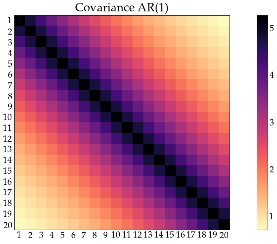
n_obs = 20
arparams = np.array([0.9])
maparams = np.array([0])
ar = np.r_[1, -arparams] # add zero-lag and negate
ma = np.r_[1, maparams] # add zero-lag
sigma2=np.array([1])

acov_ar1 = arma_acovf(ar=ar, ma=ma, nobs=n_obs, sigma2=sigma2)

Sigma_ar1 = toeplitz(acov_ar1)

corr_ar1 = correlation_from_covariance(Sigma_ar1)

show_covariance(cov_mat=Sigma_ar1, process_name='AR(1)')

MA and AR processes in Python

from statsmodels.tsa.arima_process import ArmaProcess

# create a MA(1) model
theta = np.array([.4])
ar = np.r_[1] # the coefficient on $z_t$
ma = np.r_[1, theta] 
ma1_process = ArmaProcess(ar, ma)

print(ma1_process)

ArmaProcess
AR: [1.0]
MA: [1.0, 0.4]

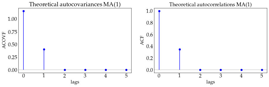
autocovariances and autocorrelations (MA models)

ma1_process.acovf(3)

array([1.16, 0.4 , 0.  ])

#compare to analytical result
print([1*(1+theta**2), theta])

[array([1.16]), array([0.4])]

def plot_autocov(process, nlags, process_name):
    lags = np.arange(nlags+1)
    acovf_x = process.acovf(nlags+1)
    acf_x = process.acf(nlags+1)

    fig, (ax1, ax2) = plt.subplots(nrows=1, ncols=2, figsize=(15, 4))
    
    ax1.vlines(lags, [0], acovf_x, color='b')
    ax1.scatter(lags, acovf_x, marker='o', c='b')
    ax1.axhline(color='black', linewidth=.3)
    ax1.set_xticks(lags)
    ax1.set_xlabel('lags', fontsize=16)
    ax1.set_ylabel('ACOVF', fontsize=16)
    ax1.set_title(f'Theoretical autocovariances {process_name}', fontsize=20)
    

    ax2.vlines(lags, [0], acf_x, color='b')
    ax2.scatter(lags, acf_x, marker='o', c='b')
    ax2.axhline(color='black', linewidth=.3)
    ax2.set_xticks(lags)
    ax2.set_xlabel('lags', fontsize=16)
    ax2.set_ylabel('ACF', fontsize=16)
    ax2.set_title(f'Theoretical autocorrelations {process_name}', fontsize=18)

def plot_sample(z, process_name):

    fig, ax = plt.subplots(figsize=(12,4))
    ax.plot(z, c='black')
    ax.set_xlabel('time', fontsize=16)
    ax.set_title(f'{process_name}', fontsize=18)

plot_autocov(process=ma1_process, nlags=5, process_name='MA(1)')

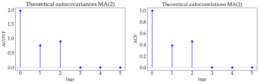
# define a MA(2) model

theta = np.array([.4, .9])
ar = np.r_[1] # the coefficient on $z_t$
ma = np.r_[1, theta] 
ma2_process = ArmaProcess(ar, ma)
plot_autocov(process=ma2_process, nlags=5, process_name='MA(2)')

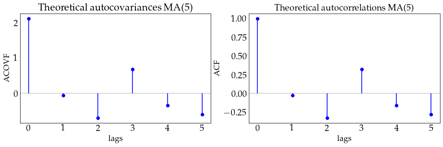
# define a MA(5) model
theta = np.array([.4, -.7, .3, -.1, -.6])
ar = np.r_[1] # the coefficient on $z_t$
ma = np.r_[1, theta] 
ma5_process = ArmaProcess(ar, ma)
plot_autocov(process=ma5_process, nlags=5, process_name='MA(5)')

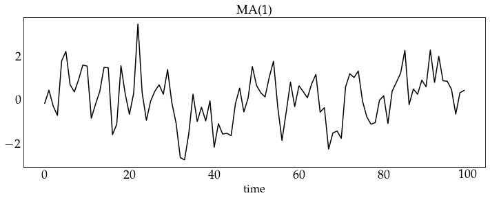
# generate a sample from the MA(1) model and plot it
z_ma1 = ma1_process.generate_sample(100)
plot_sample(z_ma1, process_name='MA(1)')

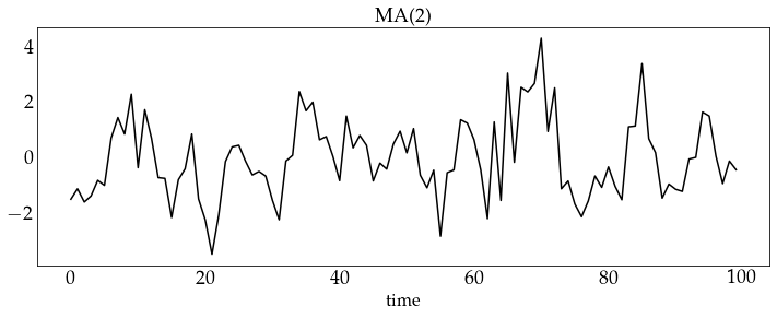
# generate a sample from the MA(2) model and plot it
z_ma2 = ma2_process.generate_sample(100)
plot_sample(z_ma2, process_name='MA(2)')

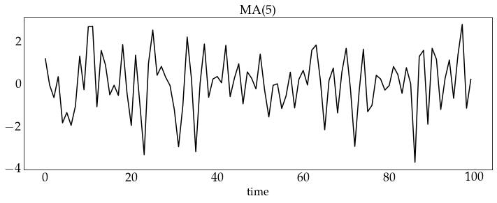
# generate a sample from the MA(5) model and plot it
z_ma5 = ma5_process.generate_sample(100)
plot_sample(z_ma5, process_name='MA(5)')

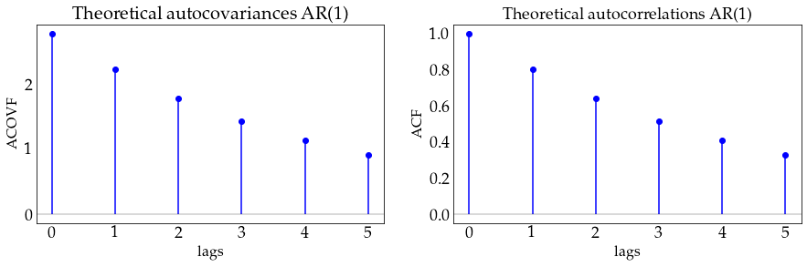
autocovariances and autocorrelations (AR models)

alpha = .8 # coefficient on z(t-1)
ar = np.r_[1, -alpha] 
ma = np.r_[1] # coefficient on e(t)
ar1_process = ArmaProcess(ar, ma)

print(ar1_process)

ArmaProcess
AR: [1.0, -0.8]
MA: [1.0]

ar1_process.acovf(3)

array([2.77777778, 2.22222222, 1.77777778])

#compare to analytical result
sigma=1
print([sigma**2 / (1-alpha**2), \
       alpha*sigma**2/(1-alpha**2), \
       alpha**2*sigma**2/(1-alpha**2)
      ])

[2.7777777777777786, 2.222222222222223, 1.7777777777777788]

plot_autocov(process=ar1_process, nlags=5, process_name='AR(1)')

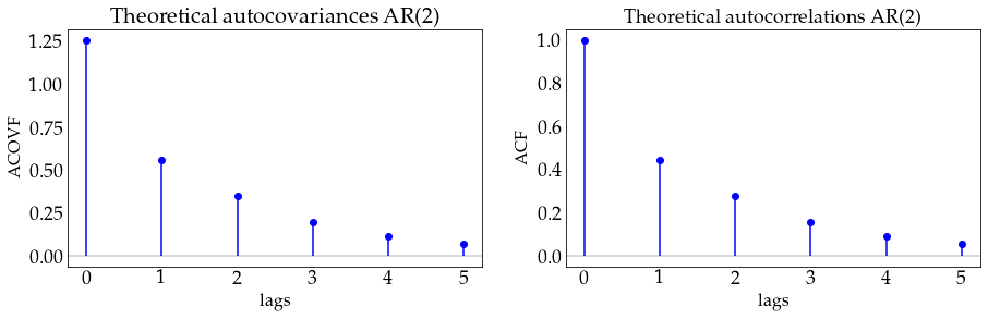
alpha = np.array([.4, .1]) 
ar = np.r_[1, -alpha] # the coefficient on $z_t$
ma = np.r_[1] 
ar2_process = ArmaProcess(ar, ma)
plot_autocov(process=ar2_process, nlags=5, process_name='AR(2)')

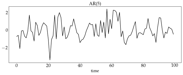
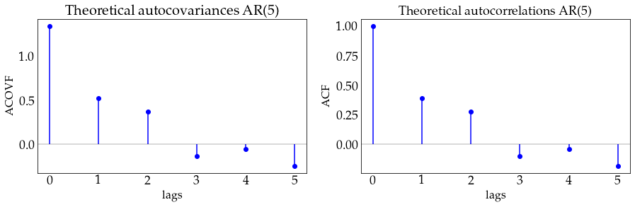
alpha = np.array([.4, .2, -.3, .1, -.1])
ar = np.r_[1, -alpha] # the coefficient on $z_t$
ma = np.r_[1] 
ar5_process = ArmaProcess(ar, ma)
plot_autocov(process=ar5_process, nlags=5, process_name='AR(5)')

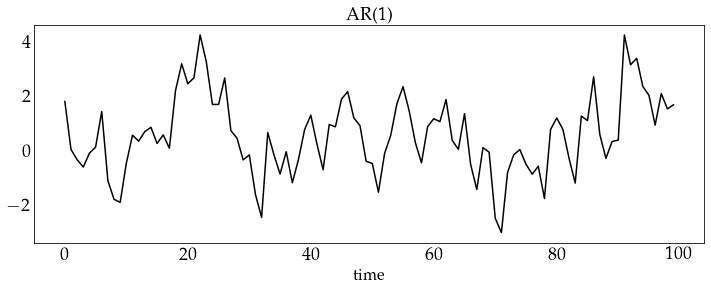
z_ar1 = ar1_process.generate_sample(100)
plot_sample(z_ar1, process_name='AR(1)')

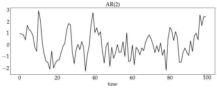
z_ar2 = ar2_process.generate_sample(100)
plot_sample(z_ar2, process_name='AR(2)')

z_ar5 = ar5_process.generate_sample(100)
plot_sample(z_ar5, process_name='AR(5)')

Non-zero mean

MA(1)

$$z_t=\mu +{\epsilon }_t+\theta {\epsilon }_{t-1}$$

$$\mathrm{E}(z_t)=\mu$$

AR(1)

$$z_t={\alpha }_0+{\alpha }_1{z}_{t-1}+{\epsilon }_t$$

$$\mathrm{E}(z_t)=\mu$$

$$\begin{array}{r}\begin{array}{rl}\mu & ={\alpha }_0+{\alpha }_1\mu \\ & =\frac{{\alpha }_0}{1-{\alpha }_1}\end{array}\end{array}$$

$$z_t-\mu ={\alpha }_1(z_{t-1}-\mu )+{\epsilon }_t$$

previous

ARMA models

next

Algebra of AR, MA models