.ipynb .pdf

Binder

Contents

Non-stationarity and unit root processes

import warnings
warnings.simplefilter("ignore", FutureWarning)

from statsmodels.tsa.deterministic import DeterministicProcess
import pandas as pd
import numpy as np

from numpy.random import default_rng
from statsmodels.tsa.arima_process import arma_acovf, ArmaProcess
from statsmodels.tsa.arima.model import ARIMA
import matplotlib.pyplot as plt
import statsmodels.api as sm
gen = default_rng(1)
import seaborn as sns
sns.set_theme()
sns.set_context("notebook")

Why need stationarity?

• stationarity is a form of constancy of the properties of the process (mean, variance, autocovariances)

• needed in order to be able to learn something about those properties

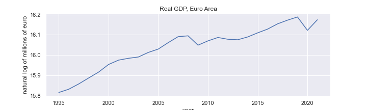
Many macroeconomic time series are non-stationary

#df = pd.read_excel('nama_10_gdp__custom_2373104_page_spreadsheet.xlsx',
#                   sheet_name='Sheet 1',
#                  skiprows=range(9), usecols=[0,1], names=['year', 'GDP'], index_col=0, parse_dates=True,
#                  ).loc['1995':'2021']
#df = df.astype('float')
#data = np.log(df['GDP'])
#title='Real GDP, Euro Area'
#ylabel='natural log of millions of euro'
#fig = data.plot(figsize=(10,3), title=title,ylabel=ylabel)
#plt.savefig('images/rGDPea.png')

ARMA(p, q)

$$z_t={\alpha }_1{z}_{t-1}+{\alpha }_2{z}_{t-1}+\cdots +{\alpha }_p{z}_{t-p}+{\epsilon }_t+{\beta }_1{\epsilon }_{t-1}+\cdots +{\beta }_q{\epsilon }_{t-q}$$

in lag operator notation

$$\begin{array}{rl}\alpha (L)z_t& =\beta (L){\epsilon }_t\end{array}$$

ARMA(p, q) is stationary if the AR§ part is stationary, i.e. if all roots of

$$\alpha (x)=1-{\alpha }_{1}x-{\alpha }_2{x}^2-\cdots -{\alpha }_p{x}^p=0$$

are outside the unit circle ($|x|>1$)

• a non-stationary process with one root $x=1$ and the other roots $|x|>1$ is called a unit root process

• if $z_t$ is an unit root process, $\mathrm{\Delta }{z}_t=z_t-z_{t-1}=(1-L)z_t$ is stationary

$$\alpha (x)={\alpha }^{\ast }(x)(1-x)$$

and if all roots of

$${\alpha }^{\ast }(x)=1-{\alpha }_1^{\ast }x-{\alpha }_2^{\ast }{x}^2-\cdots -{\alpha }_{p-1}^{\ast }{x}^{p-1}=0$$

are outside the unit circle ($|x|>1$)

the AR part

$$\begin{array}{r}\alpha (L)z_t={\alpha }^{\ast }(L)(1-L)z_t={\alpha }^{\ast }(L)(z_t-z_{t-1})={\alpha }^{\ast }(L)\mathrm{\Delta }{z}_t\end{array}$$

• a non-stationary process whose first difference is stationary is called integrated of order one ($I(1)$)

why “integrated”:

$$\mathrm{\Delta }{z}_t=z_t-z_{t-1}=u_t,u_t\text{stationary}$$

$$\begin{array}{r}\begin{array}{rl}{z}_t& =z_{t-1}+u_t\\ & =z_{t-2}+u_{t-1}+u_t\\ & ⋮\\ & =\sum _{j=1}^t{u}_j+z_0\end{array}\end{array}$$

• $z_t$ is the sum (integral) of a process (is an “integrated” process) starting from some initialization $z_0$

• $\sum _{j=1}^t{u}_j$ refered to as a stochastic trend

• $\mathrm{\Delta }{z}_t$ is $I(0)$ (stationary, no need to difference)

• a non-stationary process which requres double difference to be stationary is called integrated of order two ($I(2)$)

  • if $z_t$ is $I(2)$ then ${\mathrm{\Delta }}^2{z}_t=(1-L{)}^2{z}_t$ is $I(0)$

• etc for $I(d)$.

  • if $z_t$ is $I(d)$ then ${\mathrm{\Delta }}^d$ is $I(0)$

  • $d$ is the order of integration

• if we difference a stationary process, we get another stationary process. However, no differencing was required to achieve stationarity

• stationary process whose cumulative sum is also stationary, are called overdifferenced, and denoted with $I(-1)$

example:

$$z_t={\epsilon }_t-{\epsilon }_{t-1},{\epsilon }_t\sim \text{iid}(0,{\sigma }^2)$$

• $z_t$ is stationary but so is ${\epsilon }_t$

• $z_t$ is $I(-1)$

• non-invertible MA part

another example:

$$z_t={\delta }_0+{\delta }_{1}t+{\nu }_t\text{with stationary }{\nu }_t$$

$$\mathrm{\Delta }{z}_t={\delta }_{1}t-{\delta }_1(t-1)+\mathrm{\Delta }{\nu }_t={\delta }_1+\mathrm{\Delta }{\nu }_t$$

is $I(-1)$

• linear time trend (deterministic trend)

• $z_t$ is called trend-stationary process

in the sense that it is non-random

more generally:

$$z_t={{\mathbf{x}}_{\mathbf{t}}}^{\prime }\delta +{\nu }_t\text{with stationary }{\nu }_t,\mathrm{E}{\nu }_t=0$$

where ${\mathbf{x}}_{\mathbf{t}}$ are known constants

$$z_t-{{\mathbf{x}}_{\mathbf{t}}}^{\prime }\delta ={\nu }_t$$

is stationary

Gaussian MLE

and, if ${\nu }_t$ is stationary Gaussian time series process

$$\mathit{\nu }\sim \mathcal{N}(\mathbf{0},\mathrm{\Sigma })$$

we have

$$\mathbf{z}\sim \mathcal{N}(\mathit{\mu },\mathbf{\Sigma })$$

where

$$\mu =\mathit{X}\delta$$

for example, if $z_t={\delta }_0+{\delta }_{1}t+{\nu }_t$, the $t$-th row of $\mathit{X}$ is $[1,t]$

Models with time trend in Python

Generate $\mathit{X}$ for

$$z_t={\delta }_0+{\delta }_{1}t+{\nu }_t,t=1,2,\cdots ,T$$

$$\mathbf{z}=\mathit{X}\delta +\nu$$

$T\times 2$ matrix with $t$-th row given by $[1,t]$

from statsmodels.tsa.deterministic import DeterministicProcess

T = 500
index = pd.RangeIndex(0, T)
det_proc = DeterministicProcess(index, constant=True, order=1) # constant and a linear (1 order) trend
X = det_proc.in_sample()
X.head()

	const	trend
0	1.0	1.0
1	1.0	2.0
2	1.0	3.0
3	1.0	4.0
4	1.0	5.0

$$\mathbf{z}=\mathit{X}\delta +\nu$$

# constant and time trend part
delta = np.array([3, .1])
exog = X.values@delta 

${\nu }_t$ as ARMA(1,1) process

alpha = np.array([.8])
beta = np.array([0.1])
ar = np.r_[1, -alpha] # coefficient on z(t) and z(t-1)
ma = np.r_[1, beta]  # coefficients on e(t) and e(t-1)
arma11_process = ArmaProcess(ar, ma)

nu =  arma11_process.generate_sample(T, distrvs=gen.normal)

z = exog + nu

Option 1 Estimate indicating constant and time trend

arma_model = ARIMA(z, order=(1, 0, 1), trend="ct")
arma_results = arma_model.fit()
print(arma_results.summary())

                               SARIMAX Results                                
==============================================================================
Dep. Variable:                      y   No. Observations:                  500
Model:                 ARIMA(1, 0, 1)   Log Likelihood                -733.673
Date:                Mon, 28 Mar 2022   AIC                           1477.345
Time:                        10:48:25   BIC                           1498.418
Sample:                             0   HQIC                          1485.614
                                - 500                                         
Covariance Type:                  opg                                         
==============================================================================
                 coef    std err          z      P>|z|      [0.025      0.975]
------------------------------------------------------------------------------
const          3.0500      0.512      5.954      0.000       2.046       4.054
x1             0.0992      0.002     57.573      0.000       0.096       0.103
ar.L1          0.7971      0.035     22.981      0.000       0.729       0.865
ma.L1          0.0650      0.057      1.142      0.253      -0.047       0.176
sigma2         1.1054      0.073     15.235      0.000       0.963       1.248
===================================================================================
Ljung-Box (L1) (Q):                   0.00   Jarque-Bera (JB):                 0.28
Prob(Q):                              1.00   Prob(JB):                         0.87
Heteroskedasticity (H):               1.20   Skew:                            -0.01
Prob(H) (two-sided):                  0.24   Kurtosis:                         2.89
===================================================================================

Warnings:
[1] Covariance matrix calculated using the outer product of gradients (complex-step).

Option 2 Estimate providing exogenous regressors

$$\mathbf{z}=\mathit{X}\delta +\nu$$

arma_model2 = ARIMA(z, exog=X, order=(1, 0, 1), trend="n")
arma_results2 = arma_model2.fit()
print(arma_results2.summary()) 

                               SARIMAX Results                                
==============================================================================
Dep. Variable:                      y   No. Observations:                  500
Model:                 ARIMA(1, 0, 1)   Log Likelihood                -733.673
Date:                Mon, 28 Mar 2022   AIC                           1477.345
Time:                        10:48:29   BIC                           1498.418
Sample:                             0   HQIC                          1485.614
                                - 500                                         
Covariance Type:                  opg                                         
==============================================================================
                 coef    std err          z      P>|z|      [0.025      0.975]
------------------------------------------------------------------------------
const          3.0500      0.512      5.954      0.000       2.046       4.054
trend          0.0992      0.002     57.573      0.000       0.096       0.103
ar.L1          0.7971      0.035     22.981      0.000       0.729       0.865
ma.L1          0.0650      0.057      1.142      0.253      -0.047       0.176
sigma2         1.1054      0.073     15.235      0.000       0.963       1.248
===================================================================================
Ljung-Box (L1) (Q):                   0.00   Jarque-Bera (JB):                 0.28
Prob(Q):                              1.00   Prob(JB):                         0.87
Heteroskedasticity (H):               1.20   Skew:                            -0.01
Prob(H) (two-sided):                  0.24   Kurtosis:                         2.89
===================================================================================

Warnings:
[1] Covariance matrix calculated using the outer product of gradients (complex-step).

Difference-stationary vs trend-stationary

$$z_t={\delta }_0+{\delta }_{1}t+{\nu }_t$$

• trend-stationary if ${\nu }_t$ is stationary

• difference-stationary if ${\nu }_t$ is a unit root process

${\nu }_t$ is a unit root process if in

$$\begin{array}{rl}\alpha (L){\nu }_t& =\beta (L){\epsilon }_t\end{array}$$

one of the roots of

$$\alpha (x)=1-{\alpha }_{1}x-{\alpha }_2{x}^2-\cdots -{\alpha }_{p+1}{x}^{p+1}=0$$

is $x=1$, and the other roots are $|x|>1$

$$\alpha (L)=(1-L){\alpha }^{\ast }(L)$$

all $p$ roots of

$${\alpha }^{\ast }(x)=1-{\alpha }_1^{\ast }x-{\alpha }_2^{\ast }{x}^2-\cdots -{\alpha }_p^{\ast }{x}^p=0$$

are $|x|>1$

$\mathrm{\Delta }{\nu }_t=(1-L){\nu }_t$ is a stationary ARMA(p, q) process

$$\begin{array}{r}\begin{array}{rl}\alpha (L){\nu }_t& =\beta (L){\epsilon }_t\\ {\alpha }^{\ast }(L)(1-L){\nu }_t& =\beta (L){\epsilon }_t\\ {\alpha }^{\ast }(L)\mathrm{\Delta }{\nu }_t& =\beta (L){\epsilon }_t\end{array}\end{array}$$

Difference-stationary process

$$z_t={\delta }_0+{\delta }_{1}t+{\nu }_t$$

• ${\nu }_t$ is an ARIMA(p, 1, q) process

• $z_t$ is an ARIMAX(p, 1, q) process (ARIMA with exogenous part - constant and time trend)

• $\mathrm{\Delta }{z}_t$ is an ARMAX(p, q) process (ARMA with exogenous part - constant)

$$\mathrm{\Delta }{z}_t={\delta }_1+\mathrm{\Delta }{v}_t$$

model $z$ as regression model with ARIMA errors

Difference between trend- and difference-stationary models

example

$$\begin{array}{r}\begin{array}{rl}{z}_t& ={\delta }_0+{\delta }_{1}t+{\nu }_t\\ {\nu }_t& =\alpha {\nu }_{t-1}+{\epsilon }_t|\alpha |\le 1\end{array}\end{array}$$

at $t+h$

$$\begin{array}{r}\begin{array}{rl}{z}_{t+h}& ={\delta }_0+{\delta }_1(t+h)+{\nu }_{t+h}\\ {\nu }_{t+h}& =\alpha {\nu }_{t+h-1}+{\epsilon }_{t+h}\end{array}\end{array}$$

forecast at $t$:

$$\begin{array}{r}\begin{array}{rl}{\mathrm{E}}_t{z}_{t+h}& ={\delta }_0+{\delta }_1(t+h)+{\mathrm{E}}_t{\nu }_{t+h}\\ {\mathrm{E}}_t{\nu }_{t+h}& ={\alpha }^h{\nu }_t\\ & \Downarrow \\ {\mathrm{E}}_t{z}_{t+h}& ={\delta }_0+{\delta }_1(t+h)+{\alpha }^h{\nu }_t\end{array}\end{array}$$

• if $|\alpha |<1$, as $h\to \mathrm{\infty }$, ${\alpha }^h\to 0$

$${\mathrm{E}}_t{z}_{t+h}={\delta }_0+{\delta }_1(t+h)+{\alpha }^h{\nu }_t\to {\delta }_0+{\delta }_1(t+h)=\mathrm{E}{z}_{t+h}$$

$$\begin{array}{r}\begin{array}{rl}\mathrm{E}{z}_{t+h}& ={\delta }_0+{\delta }_1(t+h)+\mathrm{E}{\nu }_{t+h}\\ \mathrm{E}{\nu }_{t+h}& =\alpha \mathrm{E}{\nu }_{t+h-1}+\mathrm{E}{\epsilon }_{t+h}=0\end{array}\end{array}$$

For trend-stationary processes:

• the long-run forecast is the unconditional mean of $z_t$ (mean reversion)

• the long-run forecast is independent of $z_t$

• shocks to $z_t$ have temporary impact (transitory)

• if $\alpha =1$,

$$\begin{array}{r}\begin{array}{rl}{\mathrm{E}}_t{z}_{t+h}& ={\delta }_0+{\delta }_1(t+h)+{\alpha }^h{\nu }_t\\ {\mathrm{E}}_t{z}_{t+h}& ={\delta }_0+{\delta }_1(t+h)+{\nu }_t\\ {\mathrm{E}}_t{z}_{t+h}& ={\delta }_0+{\delta }_1(t+h)+\underset{{\nu }_t}{\underbrace{z_t-{\delta }_0-{\delta }_{1}t}}\\ {\mathrm{E}}_t{z}_{t+h}& ={\delta }_{1}h+z_t\end{array}\end{array}$$

For difference-stationary processes:

• the value of $z_t$ has a permanent effect on all future forecasts

  • shocks to $z_t$ have permanent effects

• $z_t$ is expected to grow by ${\delta }_1$ every period

Martingale process

if for $\{z_t{\}}_{-\mathrm{\infty }}^{\mathrm{\infty }}$

$$\mathrm{E}(z_{t+1}|z_t,z_{t-1},\cdots )=z_t$$

$z_t$ is a martingale process, and $\mathrm{\Delta }{z}_t$ is a martingale difference process

unlike a random walk, martingale process allows for heteroskedasticity or conditional heteroskedasticity

Beveridge-Nelson decomposition

• Every difference-stationary process can be written as a sum of a random walk and a stationary component

• the effect of innovations (shocks) can be decomposed into permanent and transitory effects

• ARIMA(p,1,q)

$$\alpha (L)\mathrm{\Delta }{z}_t={\delta }_0+\beta (L){\epsilon }_t$$

• $\alpha (L)$ is invertible. Why?

• equivalently (by invertability of $\alpha (L)$)

$$\begin{array}{r}\mathrm{\Delta }{z}_t={\delta }_1+\varphi (L){\epsilon }_t\end{array}$$

$${\delta }_1=\frac{{\delta }_0}{\alpha (1)},\varphi (L)=\frac{\beta (L)}{\alpha (L)}\alpha (1)=1-{\alpha }_1-\cdots -{\alpha }_p$$

(a bit of magic here…)

Since 1 is a root of the polinomial

$$\varphi (L)-\varphi (1)$$

it can be witten as

$$\varphi (L)-\varphi (1)={\varphi }^{\ast }(L)(1-L)$$

and

$$\varphi (L)={\varphi }^{\ast }(L)(1-L)+\varphi (1)$$

where

$${\varphi }^{\ast }(L)=\frac{\varphi (L)-\varphi (1)}{(1-L)}\Rightarrow {\varphi }_j^{\ast }=-\sum _{i=j+1}{\varphi }_i$$

$$\begin{array}{r}\begin{array}{rl}\mathrm{\Delta }{z}_t& ={\delta }_1+\varphi (L){\epsilon }_t\\ (1-L)z_t& ={\delta }_1+\varphi (1){\epsilon }_t+{\varphi }^{\ast }(L)(1-L){\epsilon }_t\\ z_t& =(1-L{)}^{-1}{\delta }_1+(1-L{)}^{-1}\varphi (1){\epsilon }_t+{\varphi }^{\ast }(L){\epsilon }_t\end{array}\end{array}$$

denote $z_t^p=(1-L{)}^{-1}{\delta }_1+(1-L{)}^{-1}\varphi (1){\epsilon }_t$

then,

$$\begin{array}{r}\begin{array}{rl}(1-L)z_t^p& ={\delta }_1+\varphi (1){\epsilon }_t\\ z_t^p-z_{t-1}^p& ={\delta }_1+\varphi (1){\epsilon }_t\\ z_t^p& ={\delta }_1+z_{t-1}^p+\varphi (1){\epsilon }_t\end{array}\end{array}$$

Therefore

$$\begin{array}{r}\begin{array}{rl}{z}_t& =z_t^p+z_t^s\\ \\ & \text{where}\\ \\ z_t^p& ={\delta }_1+z_{t-1}^p+\varphi (1){\epsilon }_t\\ z_t^s& ={\varphi }^{\ast }(L){\epsilon }_t\end{array}\end{array}$$

• $z_t^p$ - permanent component (trend)

• $z_t^s$ - transitory component (cycle)

• ${\epsilon }_t$ has a permanent impact on $z_t$ through $z_t^p$

• ${\epsilon }_t$ has a transitory impact on $z_t$ through $z_t^s$

• relative importance of permanent/transitory impact depends on the value of $\varphi (1)$

example ARIMA(0,1,1)

$$\mathrm{\Delta }{z}_t={\epsilon }_t+\beta {\epsilon }_{t-1}$$

$$\begin{array}{r}\begin{array}{rl}{z}_t& =z_{t-1}+{\epsilon }_t+\beta {\epsilon }_{t-1}\\ & =z_{t-2}+({\epsilon }_{t-1}+\beta {\epsilon }_{t-2})+{\epsilon }_t+\beta {\epsilon }_{t-1}\\ & ⋮(\text{assuming }{z}_0={\epsilon }_0=0)\\ & =\sum _{j=1}^t{\epsilon }_j+\beta \sum _{j=1}^{t-1}{\epsilon }_j(\text{add and subtract }\beta {\epsilon }_t)\\ & =\underset{z_t^p}{\underbrace{(1+\beta )\sum _{j=1}^t{\epsilon }_j}}+\underset{z_t^s}{\underbrace{(-\beta {\epsilon }_t)}}\end{array}\end{array}$$

$$\begin{array}{r}\begin{array}{rl}{z}_t^p& =(1+\beta )\sum _{j=1}^t{\epsilon }_j\\ & =(1+\beta )\sum _{j=1}^{t-1}{\epsilon }_j+(1+\beta ){\epsilon }_t\\ & =z_{t-1}^p+(1+\beta ){\epsilon }_t\end{array}\end{array}$$

Random walk with a drift model:

$$z_t=\delta +z_{t-1}+{\epsilon }_t$$

$$\begin{array}{r}\begin{array}{rl}{z}_t=\delta t+{\epsilon }_t& +{\epsilon }_{t-1}+{\epsilon }_{t-2}+\cdots +{\epsilon }_1+z_0\\ \\ \mathrm{E}{z}_t& =\delta t+\mathrm{E}{z}_0\\ \mathrm{var}(z_t)& ={\sigma }^{2}t+\mathrm{var}(z_0)\end{array}\end{array}$$

Beveridge-Nelson decomposition

Every difference-stationary processes can be written as a sum of a random walk and a stationary component

• many macro variables are well represented by ARIMA(p,1,q) models

• every ARIMA(p,1,q) model has a random walk stochastic trend

$$\Downarrow$$

• the growth in macro variables can be characterized by stochastic trends

Forecasting integrated variables

• if $z_t$ is $I(1)$, we estimate and forecast using $\mathrm{\Delta }{z}_t$

• from the forecasts of $\mathrm{\Delta }{z}_{t+i}$, $i=1,2,\cdots ,h$

$$z_{t+h}^f=z_t+\sum _{i=1}^h\mathrm{\Delta }{z}_{t+i}^f$$

Detecting stochastic trends by unit root test

Unit root tests are one-sided tests:

• $H_0$: unit root

• $H_1$: stationary

Augmented Dickey–Fuller test

Consider AR(2) process:

$$z_t={\alpha }_1{z}_{t-1}+{\alpha }_2{z}_{t-2}+{\epsilon }_t$$

re-write as

$$\begin{array}{r}\begin{array}{rl}{z}_t& ={\alpha }_1{z}_{t-1}+({\alpha }_2{z}_{t-1}-{\alpha }_2{z}_{t-1})+{\alpha }_2{z}_{t-2}+{\epsilon }_t\\ & =({\alpha }_1+{\alpha }_2)z_{t-1}-{\alpha }_2(z_{t-1}-z_{t-2})+{\epsilon }_t\\ & =({\alpha }_1+{\alpha }_2)z_{t-1}-{\alpha }_2\mathrm{\Delta }{z}_{t-1}+{\epsilon }_t\end{array}\end{array}$$

and

$$\begin{array}{r}\begin{array}{rl}{z}_t-z_{t-1}& =({\alpha }_1+{\alpha }_2-1)z_{t-1}-{\alpha }_2\mathrm{\Delta }{z}_{t-1}+{\epsilon }_t\\ \mathrm{\Delta }{z}_t& =({\alpha }_1+{\alpha }_2-1)z_{t-1}-{\alpha }_2\mathrm{\Delta }{z}_{t-1}+{\epsilon }_t\end{array}\end{array}$$

For AR(2) process, unit root means that $x=1$ is a solution to

$$\alpha (x)=1-{\alpha }_{1}x-{\alpha }_2{x}^2=0$$

i.e

$$\alpha (1)=1-{\alpha }_1-{\alpha }_2=0$$

Therefore, testing for unit root is equivalent to testing that $\rho =0$ in

$$\begin{array}{r}\begin{array}{rl}\mathrm{\Delta }{z}_t& =({\alpha }_1+{\alpha }_2-1)z_{t-1}-{\alpha }_2\mathrm{\Delta }{z}_{t-1}+{\epsilon }_t\\ \\ & =\rho z_{t-1}+{\alpha }_1^{\ast }\mathrm{\Delta }{z}_{t-1}+{\epsilon }_t\end{array}\end{array}$$

In general AR§ model for $z_t$

$$\begin{array}{r}\begin{array}{rl}\mathrm{\Delta }{z}_t& =({\alpha }_1+{\alpha }_2+\cdots +{\alpha }_p-1)z_{t-1}+{\alpha }_1^{\ast }\mathrm{\Delta }{z}_{t-1}+\cdots -{\alpha }_{p-1}^{\ast }\mathrm{\Delta }{z}_{t-p+1}+{\epsilon }_t\\ \mathrm{\Delta }{z}_t& =\rho z_{t-1}+\sum _{i=1}^{p-1}{\alpha }_i^{\ast }\mathrm{\Delta }{z}_{t-i}+{\epsilon }_t\end{array}\end{array}$$

• testing for unit root is equivalent to testing that $\rho =0$

(5)$$\mathrm{\Delta }{z}_t=\rho z_{t-1}+\sum _{i=1}^{p-1}{\alpha }_i^{\ast }\mathrm{\Delta }{z}_{t-i}+{\epsilon }_t$$

• in (5) the $H_1$ is that $z_t$ is a stationary mean 0 AR§ process

• to test for unit root agains $H_1$ that $z_t$ is a stationary around a constant ($\ne 0$) mean, estimate

(7)$$\mathrm{\Delta }{z}_t={\delta }_0+\rho z_{t-1}+\sum _i^{p-1}{\alpha }_i^{\ast }\mathrm{\Delta }{z}_{t-i}+{\epsilon }_t$$

• to test for unit root agains $H_1$ that $z_t$ is a stationary around a deterministic linear time trend (trend-stationary)

(7)$$\mathrm{\Delta }{z}_t={\delta }_0+{\delta }_{1}t+\rho z_{t-1}+\sum _i^{p-1}{\alpha }_i^{\ast }\mathrm{\Delta }{z}_{t-i}+{\epsilon }_t$$

• appropriate for series that exhibit growth over the long run

The test for unit root is a test of $\rho =0$ (unit root) against the alternative of $\rho <0$ (stationary)

• The asymptotic distribution of the test statistic for $\rho$ is non-standard.

• The critical values of the test statistics are obtained by Monte Carlo simulations, and depend of whether constant and time trend are included

• The null hypothesis of a unit root is rejected when value of the test statistics is below the critical value.

• If the null hypothesis cannot be rejected, $z_t$ should be differenced prior to estimation

ADF test in Python

df = pd.read_stata(r"C:\Users\eeu227\Documents\PROJECTS\econ108-repos\econ108-practice\EconometricsData\FRED-QD\FRED-QD.dta")
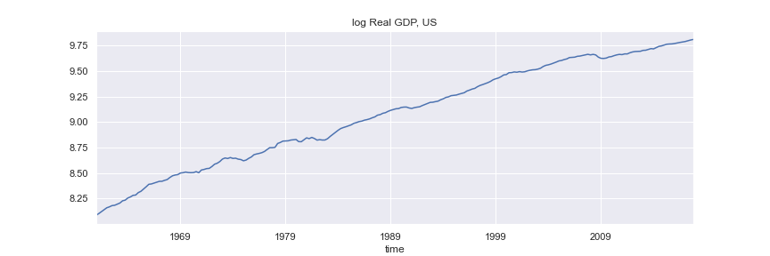
rgdp = df[['time', 'gdpc1']].set_index('time')['1961q1':].rename(columns={'gdpc1': 'rGDP'})
rgdp = np.log(rgdp)

df = pd.read_stata(r"C:\Users\eeu227\Documents\PROJECTS\econ108-repos\econ108-practice\EconometricsData\FRED-MD\FRED-MD.dta")
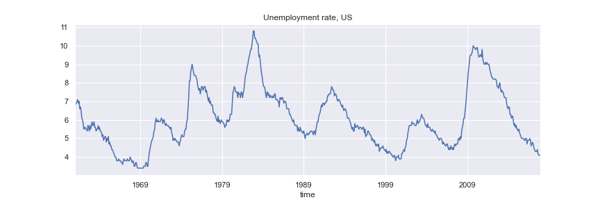
unemp = df[['time', 'unrate']].set_index('time')['1961-01':]

df = pd.read_stata(r"C:\Users\eeu227\Documents\PROJECTS\econ108-repos\econ108-practice\EconometricsData\FRED-MD\FRED-MD.dta")
cpi = np.log(df[['time', 'cpiaucsl']].set_index('time')['1961-01':])

dcpi = (cpi.diff(12)*100).dropna()

Real GDP

#fig = rgdp.plot(figsize=(12,4), title='log Real GDP, US', legend=False)
#plt.savefig('images/rGDPus.png')

from statsmodels.tsa.stattools import adfuller

def get_adfresults(dftest):
    dfoutput = pd.Series(
            dftest[0:4],
            index=[
                "Test Statistic",
                "p-value",
                "#Lags Used",
                "Number of Observations Used",
            ],
        )
    for key, value in dftest[4].items():
        dfoutput[f"Critical Value ({key})"] = value
    return dfoutput

ADF with constant and trend, 4 lags

dftest = adfuller(rgdp, maxlag=4, autolag=None, regression='ct')
dftest

(-2.0141544954585036,
 0.5937024444875985,
 4,
 223,
 {'1%': -3.9999506167815206,
  '5%': -3.4303636888103926,
  '10%': -3.138725564735756})

get_adfresults(dftest)

Test Statistic                  -2.014154
p-value                          0.593702
#Lags Used                       4.000000
Number of Observations Used    223.000000
Critical Value (1%)             -3.999951
Critical Value (5%)             -3.430364
Critical Value (10%)            -3.138726
dtype: float64

Automatically determine optimal number of lags using AIC

dftest = adfuller(rgdp, autolag="AIC", regression='ct')
get_adfresults(dftest)

Test Statistic                  -2.157741
p-value                          0.513651
#Lags Used                       2.000000
Number of Observations Used    225.000000
Critical Value (1%)             -3.999579
Critical Value (5%)             -3.430185
Critical Value (10%)            -3.138621
dtype: float64

Unemployment Rate

#fig = unemp.plot(figsize=(12,4), title='Unemployment rate, US', legend=False)
#plt.savefig('images/UNus.png')

dftest = adfuller(unemp, autolag='AIC', regression='c')
get_adfresults(dftest)

Test Statistic                  -2.996063
p-value                          0.035264
#Lags Used                      12.000000
Number of Observations Used    671.000000
Critical Value (1%)             -3.440133
Critical Value (5%)             -2.865857
Critical Value (10%)            -2.569069
dtype: float64

Consumer Price Inflation

#fig = dcpi.plot(figsize=(12,4), title='Inflation rate, US', legend=False)
#plt.savefig('images/dCPIus.png')

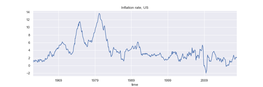
dftest = adfuller(dcpi, autolag='AIC', regression='c')
get_adfresults(dftest)

Test Statistic                  -2.804916
p-value                          0.057575
#Lags Used                      15.000000
Number of Observations Used    656.000000
Critical Value (1%)             -3.440358
Critical Value (5%)             -2.865956
Critical Value (10%)            -2.569122
dtype: float64

ADF test using ARCH

from arch.unitroot import ADF

adf = ADF(rgdp, trend="ct")
adf.summary()

Augmented Dickey-Fuller Results

Test Statistic	-2.158
P-value	0.514
Lags	2

Trend: Constant and Linear Time Trend
Critical Values: -4.00 (1%), -3.43 (5%), -3.14 (10%)
Null Hypothesis: The process contains a unit root.
Alternative Hypothesis: The process is weakly stationary.

Examine the regression results

reg_res = adf.regression
print(reg_res.summary())

                            OLS Regression Results                            
==============================================================================
Dep. Variable:                      y   R-squared:                       0.176
Model:                            OLS   Adj. R-squared:                  0.161
Method:                 Least Squares   F-statistic:                     11.76
Date:                Mon, 28 Mar 2022   Prob (F-statistic):           1.13e-08
Time:                        16:43:14   Log-Likelihood:                 786.27
No. Observations:                 225   AIC:                            -1563.
Df Residuals:                     220   BIC:                            -1545.
Df Model:                           4                                         
Covariance Type:            nonrobust                                         
==============================================================================
                 coef    std err          t      P>|t|      [0.025      0.975]
------------------------------------------------------------------------------
Level.L1      -0.0217      0.010     -2.158      0.032      -0.041      -0.002
Diff.L1        0.2365      0.065      3.611      0.000       0.107       0.366
Diff.L2        0.1917      0.066      2.923      0.004       0.062       0.321
const          0.1848      0.083      2.231      0.027       0.022       0.348
trend          0.0001    7.5e-05      1.935      0.054   -2.67e-06       0.000
==============================================================================
Omnibus:                       17.613   Durbin-Watson:                   1.994
Prob(Omnibus):                  0.000   Jarque-Bera (JB):               56.070
Skew:                          -0.116   Prob(JB):                     6.68e-13
Kurtosis:                       5.435   Cond. No.                     2.21e+04
==============================================================================

Notes:
[1] Standard Errors assume that the covariance matrix of the errors is correctly specified.
[2] The condition number is large, 2.21e+04. This might indicate that there are
strong multicollinearity or other numerical problems.

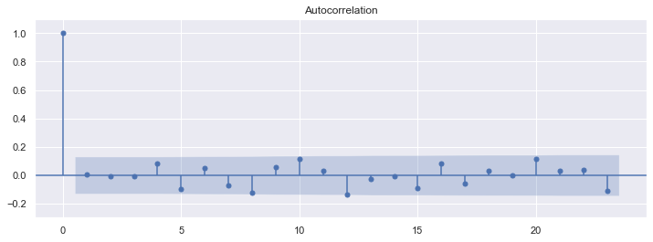
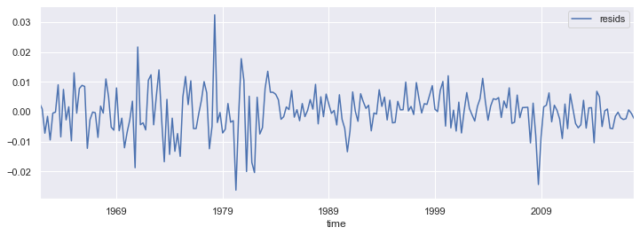
Examine the regression residuals

resids = pd.DataFrame(reg_res.resid)
resids.index = rgdp.index[3:]
resids.columns = ["resids"]
fig = resids.plot(figsize=(12,4))

fig, ax = plt.subplots(figsize=(12,4))
fig = sm.graphics.tsa.plot_acf(reg_res.resid, lags=23, ax=ax)
ax.set_ylim([-0.3, 1.1])

(-0.3, 1.1)

previous

Non-stationarity

next

Conditional Heteroskedasticity