Regime-switching models
Contents
import matplotlib.pyplot as plt
import pandas as pd
from fredapi import Fred
fred = Fred(api_key="your_api_key")

start = '1948-01'
end = '2022-01'

unr = fred.get_series('UNRATE',  observation_start=start)
unr.index.freq = unr.index.inferred_freq
unr.name = 'Unemployment'
recessions = fred.get_series('USREC',  observation_start=start, observation_end=end)
recessions.name='recessions'
df = pd.merge(unr, recessions, how='outer', left_index=True, right_index=True)
df = df.fillna(value=0)
df.index.freq = df.index.inferred_freq
dates = df.index._mpl_repr()


indpr = fred.get_series('INDPRO',  observation_start=start, observation_end=end)
indpr.index.freq = indpr.index.inferred_freq
indpr.name = 'Industrial production'
indpr = indpr.to_frame()
Regime-switching models¶
Motivation¶
empirically, economic contractions are steeper and more short-lived than expansions
fig, ax = plt.subplots(figsize=(12,6))

df[['Unemployment']].plot(ax=ax)
ylim = ax.get_ylim()
ax.fill_between(dates, ylim[0], ylim[1], df[['recessions']].values.flatten(), facecolor='k', alpha=0.1);
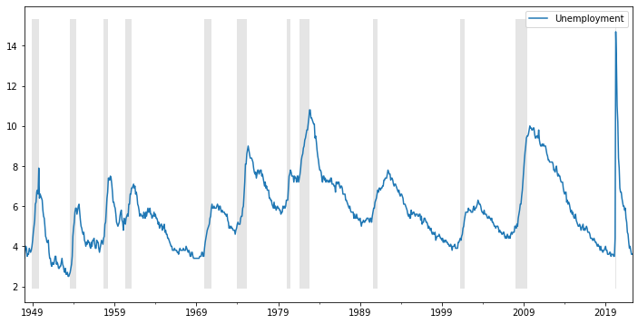
fig2, ax = plt.subplots(figsize=(12,6))

indpr.plot(ax=ax)
ylim = ax.get_ylim()
ax.fill_between(dates, ylim[0], ylim[1], df[['recessions']].values.flatten(), facecolor='k', alpha=0.1);
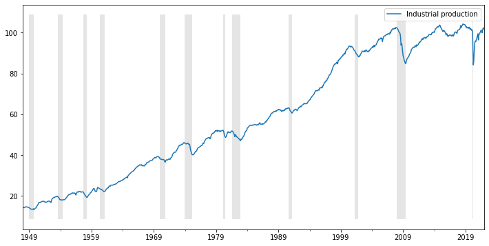
asymmetry between different phases of the business cycle
linear models rule out different dynamics of variables during contractions and expansions
contractions are much less common part of the sample
trend-cycle decompositions based on linear models are better at representing dynamics during expansions.
non-linear models may be better at capturing the business cycle asymmetry
asymmetry may be explained by different propagation mechanism in contractions vs expansions, or by asymmetry in the shocks
capacity constraints, monopoly power, downward vs upward price/wage stickiness, etc
Regime-switching AR§ model¶
if \(S_t\) is known (observed) this model can be estimated in the usual way by MLE or OLS using dummies
not very appealing as this assumes regime switches are deterministic - can be predicted
if \(S_t\) is unobserved, we cannot condition on \( S_t, S_{t-1}, ..., S_{t-p}\), and have to work with
integrate out \(S_t, S_{t-1}\) from the joint density \(p(z_t, S_t, S_{t-1} | Z_{t-1})\) by summing over all possible values of \(S_t\) and \(S_{t-1}\)
using
we have
\(p(z_t | S_t, S_{t-1}, Z_{t-1})\) computed as before (for known \(S_t\))
Hamilton filter (Hamilton (1989)):
assumes time-invariant Markov chain
what if \(p_{1,1} = 1?\)
restrictions?
computes \(\operatorname{Pr}(S_t=i, S_{t-1}=j | Z_{t-1})\) iteratively starting with the unconditional probabilities
Markov-switching models in Statsmodels¶
Two classes of models:
markov-switching dynamic regression models
where both \(x_t\) and \(y_t\) may include lags of \(z_t\)
\(z_t\) depends only on the current state (the intercept has 2 possible values for a model with 2 states)
markov-switching autoregression models
\(z_t\) depends on the current and past states (the intercept has 4 possible values for a model with 2 states when p=1)